mud pump stroke sensor free sample

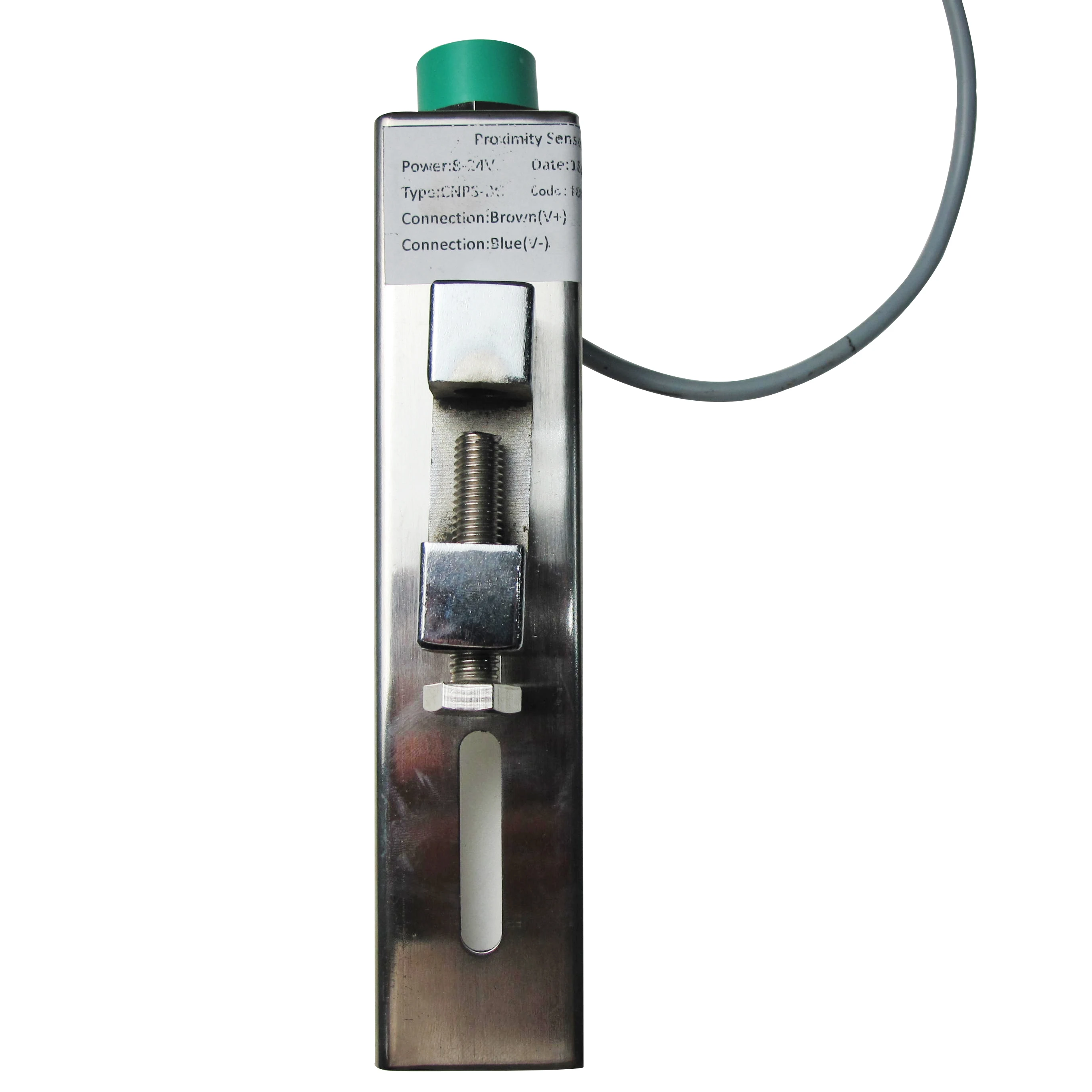
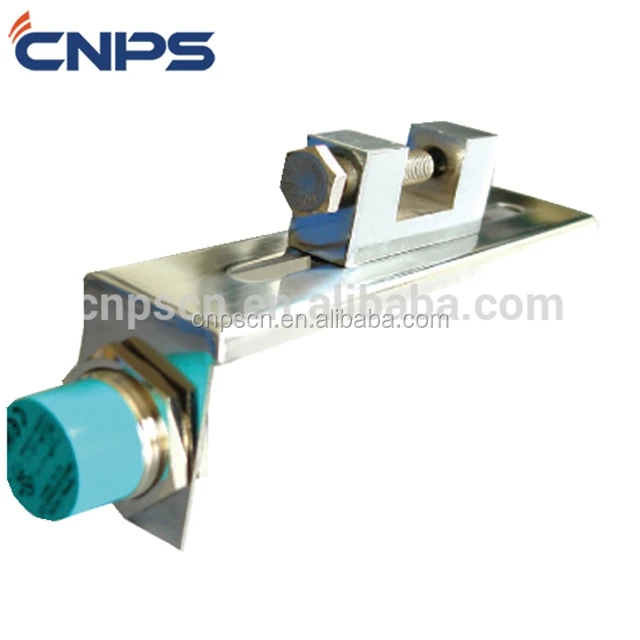
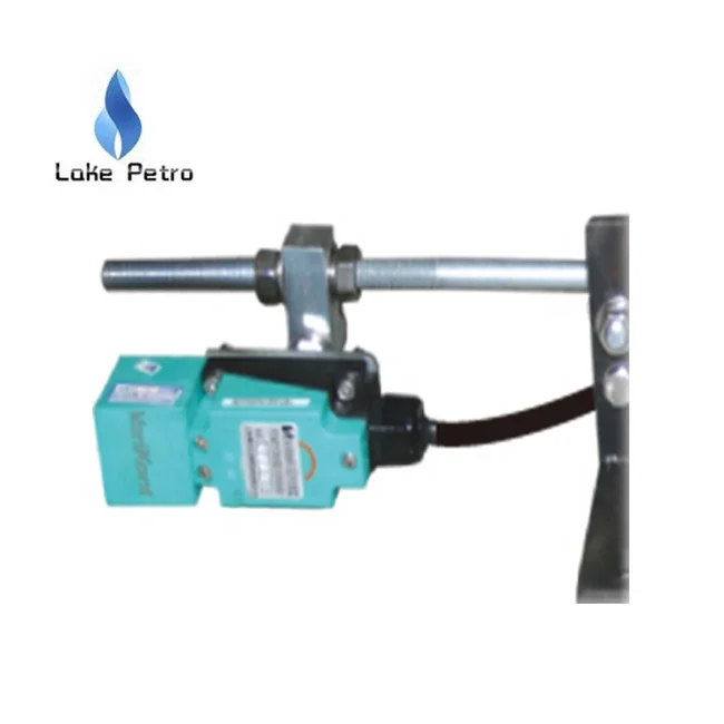
1.The pumping sensor can be fixed to the mud pump head by the bracket, or the appropriate part of the turntable, and the closest distance between the position of the sensing surface of the measured object and the end surface of the sensor is within 30 mm. (According to the influence of the use environment, the rated working distance is generally taken. 80%), plus the working voltage, when the end of the inductive sports sensor is close, the indicator light is on; when away from the sensor, the indicator is off.

2.The turntable speed sensor can be fixed to the appropriate part of the drive shaft of the turntable with the bracket. It should be convenient to install and repair. The model of the drill is selected. A piece of iron with a length and width of 30mm is welded on the shaft of the drive shaft or the airbag clutch. The position of the end face should be close to the end face of the sensor. Adjust the fixing nut of the sensor so that the distance between the iron sensor is within the effective range of the working distance.

Our pump stroke counter systems (CPS101 Series) measure the stroke rate and number of strokes on mud pumps. The oilfield pump stroke system is user-friendly and reliable and is configurable to measure up to three mud pumps at once. Our digital pump stroke counter systems are manufactured here in the U.S. by Crown Oilfield Instrumentation, and Crown’s Pump Stroke Counter provides easy monitoring of strokes per minute on multiple mud pumps. Each mud pumps’s stroke rate can be selected individually and the display is updated regularly for accurate monitoring. LCD displays indicate both pumps strokes per minute and the total number of strokes. Located at the bottom of the panel, push buttons provide easy operation and reseting of each pump. When you need to accurately monitor and maintain the amount of mud being pumped, you can trust Crown’s oilfield stroke counters.

The Magneto® Pump Stroke Sensor is the latest new product from ASD Holdings (Advanced Sensor Design). ASD has successfully introduced unique products for the Oil & Gas Industry for over a decade. In this newest creation we find that the Magneto® Pump Stroke Sensor has been patented by Advanced Sensor Design. It is the world’s first pump stroke sensor that is mounted to the outside housing of the rig pump. It is mounted and stays in place by the use of a heavy duty magnet. The Magneto PSS is completely capable of detecting and counting Oil Rig “mud pump piston strokes” without having to make or be in contact with the pistons.

It is no longer a requirement to open the covers of the Oil Rig mud pumps to install a C-clamp style micro switch with a metal whisker. (Note picture below labeled C-clamp style micro switch) No longer is it necessary to bore a hole through the pump housing in order to get a proximity switch close enough to a piston to count actual strokes. (Note picture below labeled Cable going through pump housing) The Magneto® Pump Stroke Sensor is simple to install and easy to monitor!

The magnetic base of the Magneto® PSS makes it totally different than anything available in the marketplace today relative to its form and fit. However, that is not its only outstanding feature. Advanced Sensor Design is using “State of the Art” electronic circuitry that has the ability to give the end user (Oil Rig Mud Pump Operator) an On/Off switch type electrical output. Just like what the conventional mud pump sensors emit today. The obvious benefit to the oil rig is that No Special accommodations to their Data Acquisition Systems are required.

Mud pulse telemetry (MPT) is used to transmit data from downhole instruments to the surface using drilling mud or other fluids in a borehole (e.g., the mud column) as a “communication channel”. Controlled pressure variations are used to modulate signals on top of the static mud pressure, which is generated by surface mud pumps. Pressure waves travel up to the surface, weakened by attenuation and other effects, where they are detected by one or more pressure transducers. During transmission, the pressure signals can be significantly affected by many “noise” sources. Pressure transducers are typically positioned closer to the mud pumps than to the pressure signal generators (e.g., mud pulsers), resulting in significant noise from the mud pumps in the detected signals. To attenuate the effect of the individual contributions of each piston in a mud pump, dampeners are used to smooth the pressure. Despite the use of dampeners, some pressure signal artifacts of each pump can remain and distort the MPT pressure signals.

An embodiment includes a method for transmitting data from a downhole component. The method includes: measuring a borehole fluid pressure by a receiver at a selected sampling rate and estimating a pressure signal transmitted through the fluid based on the sampled fluid pressures; measuring, by at least one pump stroke sensor, operation of a pump configured to advance fluid through the borehole; identifying individual stroke events from the pump stroke sensor measurement; generating a digital pump stroke signal in response to detecting one or more stroke events, each pump stroke signal including a digital time value associated with each of one or more stroke events; and transmitting the pump stroke signal to the receiver.

Another embodiment includes a telemetry system having: a transmitter disposed in a borehole in an earth formation, the transmitter configured to generate a pressure signal in a downhole fluid representing a communication from a downhole component; a receiver configured to measuring a borehole fluid pressure at a selected sampling rate and estimate the pressure signal transmitted through the fluid based on the sampled fluid pressures; a pump stroke sensor configured to measure operation of a pump configured to advance fluid through the borehole; and a processor configured to: identify individual stroke events from the pump stroke sensor measurement and generate a digital pump stroke signal in response to detecting one or more stroke events, the pump stroke signal including a digital time value associated with each of one or more stroke events; and transmit the pump stroke signal to the receiver.

Disclosed are systems and methods for transmitting pump stroke information and using such information to remove or reduce the effects of pump noise on fluid telemetry operations. In one embodiment, pump stroke signals are received from one or more pump stroke sensors and used to identify the position in time and/or time scale of each signature associated with a pump cycle. Pump Noise Cancellation (PNC) processing may be performed to remove the signatures from received telemetry pressure signals. One or more pump stroke sensors include or communicate with a processor configured to sample pressure measurements and transmit pump stroke signals on an event basis, i.e., in response to detecting a pump stroke event. In one embodiment, the processor generates a digital pump stroke signal including a pump identification and an event time indication, which can be used in a PNC processing algorithm. One embodiment of a PNC algorithm uses one stroke sensor and/or signal per pump, irrespective of the number of pistons per pump. The pump stroke signals and telemetry signals from a transmitter are received by a signal processing unit, which can be, e.g., a (centralized) data acquisition system or part of a smart pressure transducer. The systems and methods described herein are applicable both central processing configurations as well as distributed configurations, such as a digital sensor network, and serve to minimize transmission and communication bandwidth between sensors or other components in a telemetry system.

Referring to FIG. 1, an exemplary embodiment of a downhole drilling, exploration, completion, production and/or measurement system 10 disposed in a borehole 12 is shown. A borehole string, shown in this embodiment as a drill string 14, is disposed in the borehole 12, which penetrates at least one earth formation 16. Although the borehole 12 is shown in FIG. 1 to be of constant diameter, the borehole is not so limited. For example, the borehole 12 may be of varying diameter and/or direction (e.g., azimuth and inclination). The drill string 14 is made from, for example, a pipe, multiple pipe sections or coiled tubing. The system 10 and/or the drill string 14 includes various downhole components or assemblies, such as a drilling assembly 18 (including, e.g., a drill bit and mud motor) and various measurement tools and communication assemblies, one or more of which may be configured as a bottomhole assembly (BHA) 20. The various measurement tools may be included for performing measurement regimes such as wireline measurement applications, logging-while-drilling (LWD) applications and measurement-while-drilling (MWD) applications.

In this embodiment, the drillstring 14 drives a drill bit 22 that penetrates the formation 16. Downhole drilling fluid 24, such as drilling mud, is pumped through a surface assembly 26 (including, e.g., a derrick, rotary table and standpipe) into the drillstring 14 using one or more pumps 28, and returns to the surface through the borehole 12. Although the embodiments described herein relate to drilling and LWD applications, they are not so limited. The embodiments may be incorporated with any system in which downhole fluid introduced, such as a production system in which fluid is pumped downhole to facilitate production of hydrocarbons from a formation and/or hydraulically stimulate or fracture a formation.

In one embodiment, a logging and/or measurement apparatus 30 including one or more sensors is disposed with the drill string 14, for example, as part of the BHA 20 and/or a measurement sub. Exemplary logging apparatuses include devices implementing resistivity, nuclear magnetic resonance, acoustic, seismic and other such technologies.

A telemetry system (e.g., a mud pulse telemetry (MPT) system) is included in the system 10 for transmitting signals between downhole components and/or between a downhole component and a surface component. The telemetry system can be used in conjunction with any suitable component, such as such as the drilling assembly 18 and/or the measurement apparatus 28, and is configured to transmit signals through the downhole fluid 24.

The telemetry system includes a transmitter 32 that is configured to generate a pressure signal such as a series of pulses or other pressure modulation in the fluid 24 representing communications and/or data from the downhole components. For example, the transmitter 32 includes an electronics package 34 that receives and/or generates data from the measurement apparatus 30, such as logging data (e.g., formation measurement data or drilling parameter data). A mud pulser 36 generates pulses representing this data, and the pulses propagate through the fluid 24 to the surface. The telemetry signal generated by the transmitter 32 can be pressure fluctuations in the base band such as positive or negative pressure “pulses” or modulations of the frequency and/or phase of the pressure signal. Examples of such signals include frequency shift key (FSK), phase shift key (PSK) and amplitude shift key (ASK) signals.

A receiver 38 includes one or more sensors, such as one or more pressure transducers 40, that detects the a pressure signal, i.e., telemetry signal induced pressure changes, and generates signals that can be analyzed by a suitable processor. The processor may be incorporated in the receiver 38, e.g., as a processor 42, or be part of a separate surface processing unit 44 that receives data from the receiver 38 through a wired or wireless connection.

In acquiring telemetry communications from the downhole component, a processor such as the surface processing unit 44 or the processor 42 receives signals from the pressure transducer 40 and various other sensors. For example, a pump stroke sensor 46 measures the timing and stroke rate of the pump(s) 28 and sends this information to the processor. Exemplary pulse sensors include inductive pulse sensors such as NAMUR sensors and mechanical breakers or relays.

In one embodiment, noise cancellation (or reduction) includes removing artifacts introduced by the pump(s) 28. These pressure signal artifacts of each pump can be recognized as “signatures,” which are characteristic, finger-print like properties of each individual pump. Each pump cycle produces a recognizable pressure change pattern or signature that can be identified or calculated by, for example, filtering the pressure variations created by the pump(s). For example, as described further below the pump signatures can be calculated by identifying statistically significant noise and averaging the identified noise over multiple pump cycles.

One example of a bus network is shown in FIG. 1, which includes a field instrumentation bus 48 by which the various sensors communicate with one another and with processors. The bus 48 can be configured using any of various configurations or standards, such as Foundation Fieldbus, Profibus, Control Area Network (CAN) and others. The fieldbus endpoints (e.g. receivers 38, pump stroke sensors 46) are often located in areas which may possibly be exposed to explosive atmospheres (“hazardous area”). The instrument bus physical layer appropriate for this environment is “intrinsically safe” to avoid explosion hazards. Such physical layers for fieldbus systems are described in the IEC 61158-2 fieldbus standard.

In one embodiment, the receiver 38 is configured as a “smart” digital sensors, in which the actual acquisition of the telemetry signal and processing of the telemetry signal can be performed, including PNC processing. The receiver 38 includes a pressure sensor 40 connected to an A/D converter that is configured to sample the analog signal from the sensor at a selected rate, e.g., 1024 samples/second. Anti-aliasing and further noise reduction filtering can also be applied. In another embodiment, the receiver transmits the sampled digital signal (e.g., via the bus 48) to a dedicated acquisition device (DAQ) such as the surface processing unit 44. As the sensors are capable of A/D conversion, the sensor firmware could be expanded to also comprise decoding algorithms, which can further reduce bandwidth on communication bus channels.

FIG. 2 illustrates a method 50 of communicating with or between downhole components and/or processing communication data generated via intra-fluid telemetry, e.g., mud pulse telemetry. The method 50 includes one or more stages 51-55. Although the method 50 is described in some examples as being performed in conjunction with the system 10 and the mud pulse telemetry system described herein, the method 50 is not limited to use with these embodiments. In one embodiment, the method 50 includes the execution of all of stages 51-55 in the order described. However, certain stages may be omitted, stages may be added, or the order of the stages changed. In addition, a number of the stages can be performed concurrently or in parallel. For example, stages 52-55 may all be performed concurrently over the course of a downhole and/or telemetry operation.

In the first stage 51, a borehole string such as the drillstring 14 is disposed in the borehole, and a downhole operation is performed. Exemplary operations include drilling operations, LWD operations, wireline operations, completion operations, stimulation operations and others. Drilling mud or some other fluid 24 is circulated through the borehole 12 using one or more pumps 28.

In one embodiment, each component, e.g., the transmitter 32, the receiver 42 and the pump stroke sensor 46, includes clocks which are synchronized prior to deploying the drillstring 14 and/or prior to transmitting and receiving telemetry signals. All sensor internal sampling clocks are synchronized to an accuracy determined by the decoding and noise cancellation processing. For example, the maximum total jitter between 2 samples is approximately 200 μs, and thus the synchronization of clocks should be on the order of 10-50 μs.

In one embodiment, clock synchronization involves processing data received by one or more surface components (e.g. pressure transducer, pump stroke sensor, processing unit) into data (e.g., processable streams) that is associated with a timeline generated from timestamped events. For example, transmitter clock time values are shifted or otherwise modified based on the downhole tool clock drift.

It is noted that although only one transmitter 32, receiver 42 and pump stroke sensor 46 is shown, the method 50 is not limited to such a configuration. For example, the system 10 may have multiple transmitters 32 and/or receivers 42, or the system may include multiple pumps 28 and multiple associated pump stroke sensors 46.

In the second stage 52, the transmitter 32 generates a series of pulses via, for example, the mud pulser 36. A receiver 38 at a surface location (or alternatively at a remote downhole location) receives the series of pulses (i.e., the “pulse signal”) via, for example, the pressure transducer(s) 40.

In the third stage 53, a stroke sensor 46, e.g., an inductive proximity stroke sensor, measures stroke events generated by the pump 26. The stroke sensor 40 may include an A/D converter to sample the stroke sensor signal and convert it to a digital signal, or send an analog signal to another processor for sampling and conversion. For example, a digital pump stroke junction box can be used to connect a number of “n” pump stroke sensors.

Instead of sampling the stroke sensor 46 and generating a digital signal at the same sampling rate as the receiver (e.g., 1024 samples/second), the stroke sensor 46 generates and sends stroke information in an “event based” manner. In other words, the stroke sensor detects an “event” by detecting movement of various pump components (e.g., the piston) during a pump stroke and sends this information based on detecting the stroke event. In one embodiment, the stroke sensor 46 includes at least one proximity sensor. If the piston (or other pump component) passes by the stroke sensor 46, coming closer than the sensor"s proximity sensitivity, the sensor 46 indicates this “proximity” by a binary signal change. Once the piston (or other component) moves away or passes the sensor, the sensor again indicates this by the opposite logical signal (e.g., 1, 0, high, low, current, no current, etc.) The movement can be, for example, a linear movement or a rotation.

For example, the stroke sensor measures an output signal (e.g., a current amplitude curve) and generates an on/off signal per time unit (some fraction of a second). For each time unit which an “on” signal (e.g., a logical “on” signal) is generated, i.e., a stroke event is detected, the sensor generates a stroke signal including the time of the event and, in one embodiment, a pump identifier (e.g., a pump number). For each pump stroke event, a stroke signal is generated and may be sent to the processor. In one embodiment, the stroke signal includes an identification of the pump if there are multiple pumps (e.g., a pump number) and a time value of the stroke event. A “stroke event” as described herein may include a full stroke, i.e., a full pump cycle, or may include a number of strobes or impulses that make up a full stroke.

In one embodiment, the sensor element itself within the stroke sensor can signal an event without further processing or sampling the stroke sensor signal. For example, the stroke sensor is configured to change polarity in response to movement or rotation of pump components. Indication of an event may then be triggered by the polarity change of the sensor signal, producing a time-based digital event signal.

In the case of the stroke sensor 46 including a proximity sensor, the proximity sensor may produce one or more impulses (also referred to as strobes) for each pump stroke. For example, if the proximity sensor is located near the center of the pump piston movement, the sensor may detect two impulses per pump stroke or crankshaft rotation. If the sensor is located near an end of the piston, the sensor may detect one impulse per pump stroke. Depending on the sensor"s location, the movement of various components (e.g., the crankshaft, nuts or bolts) can cause additional impulses. A calibration factor associated with the number of impulses per pump stroke may thus be included in the stroke signal if necessary.

For example, a normalized pump stroke indicates exactly one crankshaft revolution. Pump speeds vary, but are usually in the order of 0-300 SPM (strokes per minutes), resulting in 0-5 stroke impulses per second for each pump. Based on synchronized sensor clocks, the stroke signal indicating the stroke event to be sent to the processor includes the pump number (or other type of pump identification) and the time of the event (stroke time). Stroke time can be an absolute time stamp or a relative time stamp (e.g. elapsed microseconds until power on or any other repeatable, high resolution time based tagging mechanism). If there are between one and five pumps per rig and a timestamp of 16 or 32 bits, the total required bandwidth for a stroke event is 3 bytes (1 byte for the pump number and 2 bytes for a 16-bit timestamp) or 5 bytes (1 byte for the pump number and 4 bytes for a 32-bit timestamp) per event. Thus, the total payload bandwidth per pump at a pump speed of 0-300 SPM (0-5 strokes/s) is less than or equal to 25 bytes/s. This is of course significantly less than a bandwidth of 1024 bytes/s or 1 kB/s if the pump stroke is sampled at the same rate as the sampling rate of the receiver 38.

A stroke signal can be sent individually for each stroke event, or multiple signals can be bundled and sent together. For example, the stroke sensor 46 or junction box can signal individual stroke events or, to further reduce the bandwidth, can send an array of stroke events every fixed number of seconds (or fractions thereof). This way multiple stroke events can be packaged into a single communication event, thereby further eliminating communication overhead.

In the fourth stage 54, the processor (e.g., the processor 42 or the surface processing unit 44) unit receives the telemetry pressure signal (e.g., mud pressure signal) as a digital signal (sampled at a selected sampling rate) or samples the analog signal at a selected sampling rate, and also receives stroke event signals from the stroke sensor 46. Each stroke event is applied to the telemetry pressure signal based on the time of the event provided by the stroke sensor, and is used to identify the time position and time interval for the pump signature (characteristic pressure variation) for each pump. The pump events are then used to analyze and/or process the telemetry pressure signal. For example, the pump events are used to reduce or eliminate via pump noise cancellation (PNC) algorithms.

Inside the receiving pressure sensor, the pressure signal may be buffered with acquisition time references dictating a maximum time period “Tbuffer,max” for acquisition of each pressure signal (e.g. 5 seconds). When the stroke signal is received, the stroke event time is used to signal and relate the beginning of a crank shaft revolution. This information can be used as part of a suitable PNC cancellation algorithm for removal of signatures from one or more pumps from pressure signals measured by the receiver 38.

Although the “events” described above are described as pump strokes, impulses or strobes, they are not so limited. The events can be any recurring or identifiable change in a component (e.g., rotational or vibrational movement) that causes changes in pressure or flow during transmission of telemetry signals. Such events can introduce noise into the telemetry signal or introduce other (e.g., desirable) effects on the telemetry signal. In addition, the events need not be recurring or be considered noise. Measurement of such events facilitates identification of the “signature” (mark or effect) on the telemetry signal. The methods described herein can be used to identify and transmit information relating to any pressure event that is to be monitored.

Upon receiving pulse signals and event information, to reduce the mud pumps" distortion of the mud pulse signal due to their signatures, the processor may perform a PNC method or algorithm to subtracting the accumulated signatures of all pumps from the pulse signal. This effectively and efficiently reduces the “noise” of the pressure signal and helps to successfully decode the telemetry information.

In the fifth stage 55, the pressure signal (from which pump signatures have been removed) is decoded to read the data transmitted by the transmitter 32.

An example of a PNC algorithm is described in conjunction with FIGS. 3-5. A “pump subtraction filter” is used to remove artifacts from pressure signals caused by mud pumps from pulse signal data. This is done by identifying and subtracting from the signal any components which recur at the same rate as the pump"s crankshaft rotation. The algorithm removes from the pulse signal data any pump-derived components, whether they are traveling downward from the pump or reflected back upstream towards the pump. The algorithm is further described in U.S. Pat. No. 4,642,800, issued Feb. 10, 1987, the entirety of which is hereby incorporated by reference.

The algorithm uses inputs from telemetry receivers such as the receiver 38, as well as pump stroke information received from the stroke sensor 46. In one embodiment, the pump stroke information includes a number of pump stroke signals, each signal including a pump identifier (if necessary) and a time value of each pump stroke event (referred to herein as a “strobe”) per pump stroke. If multiple strobes are indicated, the pump stroke signal may include a calibration factor.

In the example described herein, the pump strobe is derived from the stroke sensor 46 including a proximity switch attached to the mud pump, which senses a piston position and produces a signal once per crankshaft revolution. One pump strobe input is provided to the algorithm for each pump which might be feeding a borehole.

In this example, the inputs are received via an input data channel, which may be a pressure channel, or a flow meter output, or a combination of the two such as the output from an inference process. The algorithm may be used for a single pump and/or data channel, or may be used for any number of pumps and data channels (e.g., 1-4 data channels and 1-4 active pumps).

Output data is delivered via output channels, which typically correspond to the input data channels. In one embodiment, output data becomes available in bursts, typically around one second in length, because processing does not proceed until a pump strobe is received. It is also useful for the current state of each pump signature (one signature per pump) to be made available as output. This gives insight into the condition of the pumps.

The algorithm operates by maintaining a record of the signature of each pump. The signature corresponds to the pressure change measured associated with one pump stroke or crankshaft rotation, the time length of which can be measured using the time value of each strobe or stroke signal provided by the stroke sensor 46. The signature can be measured in the absence of telemetry signals to give an estimate of the pump contribution. In one embodiment, the pump signature is estimated by stacking or averaging a number of data sets, each data set being partitioned according to the stroke length. If multiple pumps are utilized, one signature per pump is maintained.

In order to remove the pump contribution from measured data, the signature of each active pump is subtracted from the telemetry pulse signal measured by the receiver 38, leaving a residual. When signatures of all active pumps have been subtracted, the resulting clean residual provides the output from the filter.

In order to account for variations in pump speed, after the pump signature is removed from measured data over a time interval, the signature is resampled or otherwise modified to change the time length of the signature. The change in time length can be ascertained based on the time interval of the next stroke signal. For example, suppose that the filter is running at a sample rate of 1024 per second, and that there is one pump running at 120 rpm. One crankshaft revolution (and therefore one time interval) therefore occupies 512 samples, and the pump signature is 512 samples in length. If the pump speed were to be instantaneously changed to 128 rpm, the signature would then be 480 samples in length. Before subtracting the pump signature from the new time interval, the signature would be resampled from a length of 512 to 480 samples. In practice, changes in pump rate tend to be gradual, and the resampling usually involves a change in signature length of only one or two samples.

The method 60 includes receiving a sample (block 61), and for each pump determining whether a strobe has been received within the sample time interval (block 62). If a strobe has been received, it is determined whether the pump is on (block 63). In a first instance, if a strobe was received and the pump is off, the pump is turned on (block 64). In a second instance, if a strobe was received and the pump is on, it is determined whether there are more pumps for which a strobe should be received (block 65). When a strobe is received for all pumps, sample processing (block 66) can be commenced to reduce or remove pump noise (as described, for example, in conjunction with FIGS. 4-5).

If no strobe has been received, it is determined whether the pump is on (block 67). In a third instance, if the pump is on and has not timed out (block 68), the algorithm stops until a strobe is received. In a fourth instance, if the pump has timed out, the pump is turned off (block 69). In a fifth instance, no strobe is detected and the pump is off.

If one or more pumps fall into the first, fourth or fifth instances, then some housekeeping and updating of pointers will be required. If all pumps fall into the third instance, then no additional processing is required for this sample. Detailed noise cancellation processing is generally required only when an active pump (a pump which is already on) has received a strobe, as in the second instance described above.

FIG. 5 illustrates an algorithm or method 70 for performing noise cancellation for data measured where multiple pumps are running at different speeds. Strobe processing is more complex relative to processing for a single pump, because when multiple pumps are running at different speeds it is necessary to wait for a clean residual before updating and subtracting signatures.

Strobes are held in a queue; in many cases there may be no more than two strobes in the queue, indicating the start and end of a crankshaft cycle. However, there is provision for a longer queue in case one pump runs much faster than another, in which case strobes from the faster pump must be held until the slow pump completes its crankshaft revolution and the strobes can be cleared. Strobe processing is performed when a pump has more than one strobe in its queue (i.e. at least enough to define the beginning and end of a pump cycle), and when the first strobe in its queue represents the maximum valid output, i.e. the time up to which residuals are clear. The method 70 is described in conjunction with FIG. 5, which is an exemplary time line showing strobe arrivals from a fast pump and a slow pump. Strobes A, C, D, F and G represent times of strobes for the fast pump, and strobes B, E and H represent times of strobes for the slow pump. These strobes are identified using the pump stroke signal(s) generated as described above. Each pump is also associated with a respective signature.

In the example shown in FIG. 5, the present time is between C and D. The fast pump signature has been subtracted from interval AC, and the slow pump signature has been subtracted from the interval ending at time B. The most recent strobe from the fast pump is C, and the most recent strobe from the slow pump is B. The maximum valid output is B, which is the earliest among the “most recent” strobes from the various pumps. The “maximum valid output” represents the time up to which the residual is clean, i.e., the portion of the pressure signal from which both the fast and slow pump signatures have been removed; in this example, the residual is clean up to time B.

When a strobe is received (block 71), the strobe is added to a queue for the associated pump (block 72). At time D, a strobe is received from the fast pump and added to the fast pump queue. Although now there is more than one strobe in the fast pump queue (block 73), there is not yet a clean residual up to time C, because the first strobe C is not a maximum valid output (block 74). Processing cannot yet continue because the fast pump signature (between C and D) cannot yet be updated using the previous residual.

When strobe E is received (block 71), the strobe E is added to the slow pump queue. The slow pump queue now includes at least two strobes B and E (block 73) and the first strobe B in its queue is at the maximum valid output time (block 74). Therefore, the slow pump signature ending at B is subtracted from the interval BE and data representing a clean residual between B and C is output (block 75). A “maximum-valid-output” pointer is then moved from B to C (block 76).

Because the output data has changes, a “keep-going” flag is set (block 77), and the strobe queues are checked to determine if further processing can be performed. In this example, processing can proceed because there is a clean residual on interval AC, so the fast pump signature is updated with a fraction of the residual on AC, and the updated signature is subtracted from the interval CD. Interval CD is output, and the maximum-valid-output pointer moves to D.

The processing continues for additional strobes until all of the measured data is processed to remove pump signatures. For example, strobe F is next received from the fast pump. The signature on CD is subtracted from interval D, the interval DE is output, and the max-valid-output pointer is moved to E. Strobe G is then received from the fast pump. This is added to the fast pump"s queue, but nothing more can be done with the fast pump until there is a clean residual on DF.

Strobe H is received from the slow pump. The signature corresponding to BE is subtracted from EH, interval EF is output, and the max-valid-output pointer moves to F. The fast pump signature DF is then subtracted from interval FG, interval FG is output, and the max-valid-output pointer moves to F.

Additional exemplary features of the procedure 70 are described. In one embodiment, the process includes variable weighting. When a signature is updated, a fraction of the clean residual is added back into the signature. This could be a fixed fraction, such as, e.g., 1/20. However, if this were done, it would take more than 20 pump cycles for the signature to be developed when the pumps are started up. Ideally, the signature should be developed rapidly when the pump first starts up, then updated at a progressively slower rate to maintain stability. The algorithm can therefore update the signature using a fraction 1/n of the previous clean residual, where n starts out with an initial value (e.g., two) and increases by some amount (e.g., one) for each update, until it reaches a maximum value (e.g., 20).

In one embodiment, the procedure includes auto-scaling, in which, as the pump speed changes, its signature is properly resampled in time. For example, when the signature is updated, if the latest strobe interval has increased or decreased, the signature is correspondingly expanded or compressed using, e.g., linear interpolation. In one embodiment, as the pump goes slower, it produces smaller pressure surges because the rate of change of flow is smaller. The algorithm can therefore adjust the amplitude of the signature each time it has to be resampled; the amplitude is inversely proportional to the signature length.

In one embodiment, the procedure includes signature mean subtraction. The pump signature represents the transient component of the measured data which is attributable to acceleration of the pump pistons. It is not intended to include a DC component. Each time a signature is resampled, just before it is subtracted from the data, it is adjusted to have a zero mean. The result is that any DC component in the original data is passed through to the output, where it may be used to determine a pumps-on condition.

In one embodiment, the procedure incorporates timeout processing. The algorithm is able to accommodate changes in pump speed. However, when a pump speed becomes very slow, it is not reasonable to expect the algorithm to hang indefinitely while waiting for a strobe. The algorithm therefore applies a timeout period (e.g., 5 seconds); if a strobe has not arrived from a particular pump within the timeout period, that pump is assumed to be turned off.

The systems and methods described herein provide various advantages over prior art techniques. For example, pump stroke signals may be transmitted and processed using a lower bandwidth relative to prior art techniques.

In typical MWD telemetry systems, pressure signals are sampled at a rate of 1024 samples/s. For calculating the mud pump pressure signatures, the pump stroke sensors are synchronously sampled at the same frequency/time resolution as the pressure sensors. The pressure signals and pump stroke signals are collected by a DAQ (Data Acquisition Box) containing the processing engine. These signals require that individual segments of the telemetry network (e.g., fieldbus segments) have a high bandwidth, requiring extra effort to realize the system and reducing the versatility of the system. The systems and method described herein address these deficiencies. Furthermore, due to the relatively low bandwidth of the decoded telemetry signals described herein, dedicated acquisition boxes (which are expensive and bulky due to their isolation barriers) can be avoided, and even full wireless systems can be built, further reducing installation effort and equipment cost.

In support of the teachings herein, various analysis components may be used, including digital and/or analog systems. The digital and/or analog systems may be included, for example, in the receiver 38, the stroke sensor 46 and/or the surface processing unit 44. The systems may include components such as a processor, analog to digital converter, digital to analog converter, storage media, memory, input, output, communications link (wired, wireless, pulsed mud, optical or other), user interfaces, software programs, signal processors (digital or analog) and other such components (such as resistors, capacitors, inductors and others) to provide for operation and analyses of the apparatus and methods disclosed herein in any of several manners well-appreciated in the art. It is considered that these teachings may be, but need not be, implemented in conjunction with a set of computer executable instructions stored on a computer readable medium, including memory (ROMs, RAMS, USB flash drives, removable storage devices), optical (CD-ROMs), or magnetic (disks, hard drives), or any other type that when executed causes a computer to implement the method of the present invention. These instructions may provide for equipment operation, control, data collection and analysis and other functions deemed relevant by a system designer, owner, user or other such personnel, in addition to the functions described in this disclosure.

With 60 years of experience and more than 3200 wells drilled in the Gulf of Mexico region, Continental Laboratories has accrued a leadership role in designing and implementing gas analysis systems for the Oil and Gas industry. Our latest generation gas detection system incorporates two different technologies into one detector. Catalytic sensors are utilized for greater accuracy when smaller percentages of hydrocarbon gases are present. When greater percentages are encountered, infrared sensor technology is utilized to measure target gasses up to 100% by volume.

Safety is our number one priority at Continental Laboratories and we have designed our gas detector to be as safe to operate as possible. We have added advanced safety features including over-temp monitoring, sensor status indicators, remote alarm capability and audible and visual alarms that are easily accessible to the operator.

This article will focus on understanding of MWD signal decoding which is transmitted via mud pulse telemetry since this method of transmission is the most widely used commercially in the world.

As a basic idea, one must know that transmitted MWD signal is a wave that travels through a medium. In this case, the medium is mud column inside the drill string to mud pumps. Decoding is about detecting the travelling wave and convert it into data stream to be presented as numerical or graphical display.

The signal is produced by downhole transmitter in the form of positive pulse or negative pulse. It travels up hole through mud channel and received on the surface by pressure sensor. From this sensor, electrical signal is passed to surface computer via electrical cable.

Noise sources are bit, drill string vibration, bottom hole assemblies, signal reflection and mud pumps. Other than the noises, the signal is also dampened by the mud which make the signal becomes weak at the time it reaches the pressure sensor. Depth also weaken the signal strength, the deeper the depth, the weaker the signal detected.

BHA components that have moving mechanical parts such as positive mud motor and agitator create noise at certain frequency. The frequency produced by these assemblies depends on the flow rate and the lobe configuration. The higher the flow rate and the higher the lobe configuration creates higher noise frequency.

Thruster, normally made up above MWD tool, tends to dampen the MWD signal significantly. It has a nozzle to use mud hydraulic power to push its spline mandrel – and then push the BHA components beneath it including the bit – against bottom of the hole. When the MWD signal is passing through the nozzle, the signal loses some of its energy. Weaker signal will then be detected on surface.

The pressure sensor on the pipe manifold detects 2 identical signals, one from the original MWD transmitter and another one comes from signal reflection, which are separated in some milliseconds. The result seen by the surface computer is the sum of those two signals. Depending on the individual signal width and the timing when the reflected signal arrives at the pressure sensor, surface computer may see a wider signal width or two identical signals adjacent to each other.

The common sources of signal reflection are pipe bending, change in pipe inner diameter or closed valve. These are easily found in pipe manifold on the rig floor. To avoid the signal reflection problem, the pressure sensor must be mounted in a free reflection source area, for example close to mud pumps. The most effective way to solve this problem is using dual pressure sensors method.

Mud pump is positive displacement pump. It uses pistons in triplex or duplex configuration. As the piston pushes the mud out of pump, pressure spikes created. When the piston retracts, the pressure back to idle. The back and forth action of pistons produce pressure fluctuation at the pump outlet.

Pressure fluctuation is dampened by a dampener which is located at the pump outlet. It is a big rounded metal filled with nitrogen gas and separated by a membrane from the mud output. When the piston pushes the mud the nitrogen gas in the dampener will be compressed storing the pressure energy; and when the piston retracts the compressed nitrogen gas in the dampener release the stored energy. So that the output pressure will be stable – no pressure fluctuation.

The dampener needs to be charged by adding nitrogen gas to certain pressure. If the nitrogen pressure is not at the right pressure, either too high or too low, the pump output pressure fluctuation will not be stabilized. This pressure fluctuation may match the MWD frequency signal and hence it disturbs decoding, it is called pump noise.

When the pump noise occurs, one may simply change the flow rate (stroke rate) so that the pump noise frequency fall outside the MWD frequency band – and then apply band pass frequency to the decoder.

The formula to calculate pump noise frequency is 3*(pump stroke rate)/60 for triplex pump and 2*(pump stroke rate)/60 for duplex pump. The rule of thumb to set up dampener pressure charge is a third (1/3) of the working standpipe pressure.

Sometime the MWD signal is not detected at all when making surface test although the MWD tool is working perfectly. This happen whenever the stand pipe pressure is the same with the pump dampener pressure. Reducing or increasing test flow rate to reduce or increase stand pipe pressure helps to overcome the problem.

When the MWD signal wave travels through mud as the transmission medium, the wave loses its energy. In other words, the wave is giving some energy to the mud.

The mud properties that are affecting MWD signal transmission is viscosity and weight. The increasing mud weight means there is more solid material or heavier material in the mud. Sometimes the mud weight increment is directly affecting mud viscosity to become higher. The MWD signal wave interacts with those materials and thus its energy is reduced on its way to surface. The more viscous the mud and the heavier the mud, the weaker the signal detected on surface.

Aerated mud often used in underbalance drilling to keep mud influx into the formation as low as possible. The gas injected into the mud acts as signal dampener as gas bubble is compressible. MWD signal suffers severely in this type of mud.

Proper planning before setting the MWD pulser gap, flow rate and pump dampener pressure based on mud properties information is the key to overcome weak signal.

The further the signal travels, the weaker the signal detected on the surface. The amount of detected signal weakness ratio compare to the original signal strength when it is created at the pulser depends on many factors, for example, mud properties, BHA component, temperature and surface equipment settings.

Rigging up sensor cables especially on the offshore rig is challenging since the cables must not create safety hazard to other people and equipment’s. Most of the time the cables must be run alongside rig’s high voltage electrical cables. The high voltage may induce sensor cables which creates continuous or temporal spiky signal in the surface decoder.

MUD LOG: A continuous analysis of the drilling mud and cuttings to determine the presence or absence of oil, gas, or water in the formations penetrated by the drill bit, and to ascertain the depths of any oil- or gas-bearing formations. (Gary et al., 1972)

Conventional mud logging is a wellsite effort that attempts to determine as rapidly as practicable, and from materials at hand, numerous subsurface conditions that are directly related to petroleum exploration and development drilling.

When a rock is penetrated by the drill bit, a quantity of rock with the fluids it contains — water, oil, and gas — is ground up, dispersed in the circulating drilling mud, and transported up the well annulus . The relative volumes of rock and fluids arriving at surface during any one sampling period will be controlled by:

The rationale for mud-logging services is that if representative samples of drilled materials are analyzed as soon as they come from the borehole, it should quickly be feasible to reconstruct the nature and composition of rocks and fluids at depth.

Two conditions prevent mud logging from achieving its ideal goal of providing immediate measurement of in situsubsurface conditions. First, none of the factors listed can be precisely measured to permit quantitative reconstruction of down-hole conditions. Second, drilling practices and analytic procedures introduce other variables into any such reconstruction. These include:

Mud logging originated as an exploration service in 1939. At that time it consisted of the extraction and gross detection of combustible gases carried to surface by circulating drilling mud. To provide this combustible gas detection service, a portion of the returning drilling mud was passed through a gas trap, where it was agitated and aerated. This mixture of air and extracted gas was then drawn by vacuum from the top of the trap to a nearby detector .The original "hot wire" gas detectors were nondiscriminating and provided a single output of total combustible gases to an analog meter calibrated in arbitrary "gas units." The operator, or mud logger,manually transcribed and plotted the readings of the detector. However, the analytical instruments initially available were relatively unwieldy and troublesome and required constant attention, adjustment, and recalibration. Consequently, operation and maintenance of gas detectors required the full-time attention of early mud loggers. Interpretation of the results or their correlation with other drilling data was the responsibility of the wellsite geologist or engineer.

The 1940s and early 1950s saw a broadening of the simple gas-logging effort as a consequence of improvements in gas analysis instruments. As transportable gas detectors became more rugged, reliable, and automated, mud-logging personnel had more free time to work with other on-site sources of information.

As a first step, mud loggers took over the drillers" traditional task of collecting and examining cuttings samples and preparing a lithology. Combining the lithology log with the combustible gas plot created the primitive formation log.

A soil gas analysis apparatus for surface oil prospecting was developed around 1938by R.L. Eoan, R.W. Crawford, and B.H. Ashe of Phillips Petroleum Company. In about 1939, G.G. Oberfell, Research Vice President, requested that this system be adapted to measure hydrocarbons in drilling mud to improve the chances of finding oil and gas in geological formations where electric logs of the time sometimes missed them. T.C. Wherry was assigned the task and he set up a laboratory in Oklahoma City to analyze muds from a well being drilled in the area. The mud was put in a pressure vessel and heated until head-space pressure reached about two atmospheres. At that point the gaseous mixture was expanded into an evacuated vessel. After cooling, the mixture was passed into a "hot wire" gas analyzer consisting of a platinum wire heated in a bridge circuit. The system was calibrated in terms of equivalent normal butane concentration in air.

My recollection of first direct, on-site use of mud logging occurred on Christmas Eve, 1940, in the Chocolate Bayou field near Alvin, Texas. The gas content in the mud began to build up and I informed the driller, who refused to believe it because he could not see or smell it in the mud. He would not stop drilling to circulate the gas cut mud. At this point I did insist that a test be made of the blowout preventer. Naturally it was found to be stuck open. The driller did agree, reluctantly, to clean it out, probably because there had been a disastrous blowout nearby earlier. A few minutes after repairs were made the well began to kick hard and would have blown out except for the now-working blowout preventor. About 20 feet of gas zone had been penetrated so that the near-blowout stuck the pipe in the hole and required an expensive fishing operation.

Two research mud logging units were fielded with good results prior to World War II. After the war, Bob Pryor built another one in a large trailer and operated it for a few years until industry picked up mud logging.

Initially, the quality of lithologic descriptions showed little improvement over those of drillers. Lithologic nomenclature often appears to have been restricted to terms like sand, hard shale, soft shale, lime, and "Annie Hydrite." Nevertheless, as experience and training of mud loggers improved, mud log geology became a first-hand record of the depths and characteristics of downhole rock types.

The drilling rig also provided another source of data — rate of penetration (ROP) — which has become a routine inclusion in formation logging. Initially, mud loggers took depth measurements from the driller"s report. Later, however, mud loggers began to attach their own sensors to the kelly and calculate depth drilled and ROP on a fine foot-by-foot scale. This was a substantial improvement over driller"s ten-foot-or-more averages. The addition of accurate penetration rate data permitted improved interpretation of rock strength and porosity. The ROP plot also encouraged visual correlations to be made between the mud log and those wireline logs that reflected rock properties related to drillability (e.g., porosity).

The final developmental step in formation logging was the introduction of tracer materials, such as calcium carbide, to the mud system and the addition of a pump stroke counter. With these, the rate of mud flow in the borehole could be measured accurately. This, in turn, provided a reliable means of estimating the lag time between penetration of a rock unit at depth and the arrival of its gases and cuttings at surface.

Since the development of formation logging, improvements have been made in gas detection capabilities through the introduction of more accurate and discriminating gas analyzers. Gas chromatography, for example, is now used routinely in formation logging to measure the con-cent rations of individual hydrocarbon compounds in mud and cuttings gases. Other analyzers, such as for hydrogen sulfide and carbon dioxide, can be added upon request to formation logging programs. Some modern formation logging units have incorporated pyroanalyzers to evaluate cuttings as petroleum source and reservoir rocks.

In the mid 1960s a major expansion in mud-logging services began as mud-logging companies became more involved in engineering and operational aspects of well drilling. The first expansion was to monitor for overpressured zones. This marked the transition to advanced mud-logging services.

The need for pressure evaluation services evolved because of improvements made in drilling techniques in the 1960s. Development of more stable drilling fluidsand mud additivesallowed for much greater control of mud density and mud properties. As a result, mud weight could be increased or decreased rapidly as needed, and also be maintained at relatively constant levels, without full-time attention and treatment. At the same time, improvements in blowout prevention technology, adjustable choke design,and well-kill capabilitiestook.

Balanced drilling — which is drilling with a minimum or with no overbalance of drilling mud density relative to the formation pressure gradient — reduced drilling mud treatment costs, improved penetration rates, and resulted in better overall conditions in borehole walls and adjacent formations.

However, these technical advances in drilling did not entirely remove the risks related to loss of well control. The penetration of abnormally high formation pressures could rapidly dilute the balanced mud system, lower the mud density, and cause the mud to surge to the surface. The stage would be set for a blowout.

As a result, the concept of "geopressure evaluation," also called "surnormal pressure recognition" or "pressure prediction," was incorporated into some mud-logging programs.

It was realized early that data directly applicable to identification of over-pressured zones could be obtained from available mud-logging techniques. Changes in penetration rate, cuttings character, and mud gas volume are examples of such indicators. Concurrently, mud-logging service companies introduced several additional wellsite geological and petrophysical techniques that improved detection of a "geopressured formation" or of a declining mud overbalance at the bottom of the borehole. These techniques provide such measurements as shale density, clay mineralogy (shale factor), mud temperature gradient, and mud pit volume. Techniques have continued to evolve to the point that pressure evaluation programs are now used routinely to select optimum casing points in overpressure transition zones in order to both control formation pressure on the wellbore and minimize excessive mud weight damage to openhole formations.

With the expansion of mudlogging services to include pressure evaluation, it became logical, if not necessary, to install sensors and central recorders that were able to measure continuously various drill rig, mud pit, and circulation system parameters. This led to the evolution of systems-monitoring and data-acquisition services that constantly monitored diverse drilling operations. This, in turn, resulted in drillers and operators improving overall rig performance and safety.

Advanced logging service continued to expand in the 1970s through theintroduction of mini- and microcomputers. While these were able to automate data acquisition and analysis systems, they could not be interfaced readily with older hydraulic or pneumatic sensors on the rig. As a result, independent electronic sensors were added to advanced mud-logging facilities.

Logging units set up to perform the types of advanced mud-logging service available in the 1970s were well equipped to act as "command" centers for nearly all engineering and drilling operations. This indeed became the case in many of the more advanced logging facilities in the late 1970s and early 1980s.

This funneling of data through one facility, the mud-logging unit, encouraged further expansion of advanced mud logging into interactive evaluation and advisory services. Mud-logging companies added new types of programs, software, and reports. Well kill, mud hydraulics, optimum drilling,and inventory control programsare examples. Specialized communications equipment also was incorporated in many advanced mud-logging units for two-way transmittal of data between the drillsite and company offices.

The 1980s introduced another expansion to interactive evaluation and advisory services — downhole measurement while drilling — commonly referred to as measurement while drilling(MWD). MWD technology involves installing common wireline logging sensors in the drillstring, a short distance above the bit. From these sensors, data are either transmitted directly to surface, generally through the mud system, or are recovered from recorders when the drillstring is pulled. Sensors are currently available for (1) directional monitoring (e.g., inclination, azimuth, tool face); (2) drill system monitoring (e.g., weight on bit, rotary torque, bottomhole pressure, mud temperature); and (3) formation evaluation (e.g., formation resistivity, mud resistivity, formation gamma ray).

While all of these advanced services are still generally classified as "mud logging," in many cases it can be seen that similarities lie only in the mode of operation-continuous monitoring in an on-site laboratory during active well drilling. In addition, availability has expanded to the point that many of the routine services and basic instruments can be acquired individually from the many smallercompanies that specialize in particular aspects of logging and supply stand-alone equipment.

ROP, lithology, shows, total combustible gas and individual hydrocarbon compounds of mud gas (and possibly cuttings gas), descriptive information, and basic geopressure plots.

With a diversity of services at hand, an operator has a number of decisions to make when selecting the types and levelof services needed for a specific drilling program. Conventional mud-logging services generally include the following capabilities:Monitoring, calculating, and plotting drill depth and drill rate;

Providing notification and interpretive functions to drilling supervisors concerning drilling events (e.g., oil show, gas kick, and mud cut); Interpreting formation log data and plots and correlating them to reference wireline logs and core data.

Supplemental services generally available and compatible with conventional mud-logging units and programs include these capabilities:Monitoring work sites for dangerous and nonhydrocarbon gases;

Based on observations published in 1983 by the Society of Professional Well Log Analysts(SPWLA) and information provided by established mud-logging service companies, a number of instruments and support systems are considered basic to a conventional mud-logging unit. These are listed below. Individual pieces of equipment may be omitted from a mud-logging unit if the functions they perform are not needed during a specific drilling program.

It also is advisable to ensure that logging personnel are sufficiently qualified and experienced both to operate and maintain the mud-logging equipment specified for the site and to assemble and interpret mud-logging data for designated geological and engineering purposes.

Surface mud pit volume sensor system for use in conjunction with the total hydrocarbon detector to provide immediate recognition of well kicks for well control and rig safety

Chemical apparatus to detect trace quantities of dissolved hydrogen sulfide in drilling mud; this includes an automatic hydrogen sulfide gas detector capable of signaling an alarm upon the appearance of such gas in the gas trap. (Generally, this is a minimal requirement; in an area of known hydrogen sulfide occurrence, more stringent safety provisions will probably be required.)

Text processing, log preparation, and related support items, such as typewriter, dyeline or electrostatic copier, drafting supplies and appropriate forms, sample bags, envelopes, boxes, shipping materials, and other materials needed in the routine of mud logging. In some modern conventional mud-logging units this function may include computer storage and plotting capabilities.

An SPWLA recommended formation mud log format is shown in. In this log, as with nearly all formation mud logs, data are presented in vertical, well-profile tracks for easy comparison with wireline and related down hole logs. Mud log headings are similar to those of other downhole logs, but they generally present information that summarizes the well at total depth(TD).

Drilling-related comments and data are also reported descriptively in this column, particularly if they may explain changes in ROP. For example, this column may include (1) bit type, diameter, and jet sizes; (2) bit-operating statistics, such as average weight on bit, rotary speed, torque, and pump pressure; and (3) final bit footage, hours, and grade. Track One commonly records trips and shut-in times, and it may carry directional survey data. This track also denotes the drilling chronology of the well by the placement