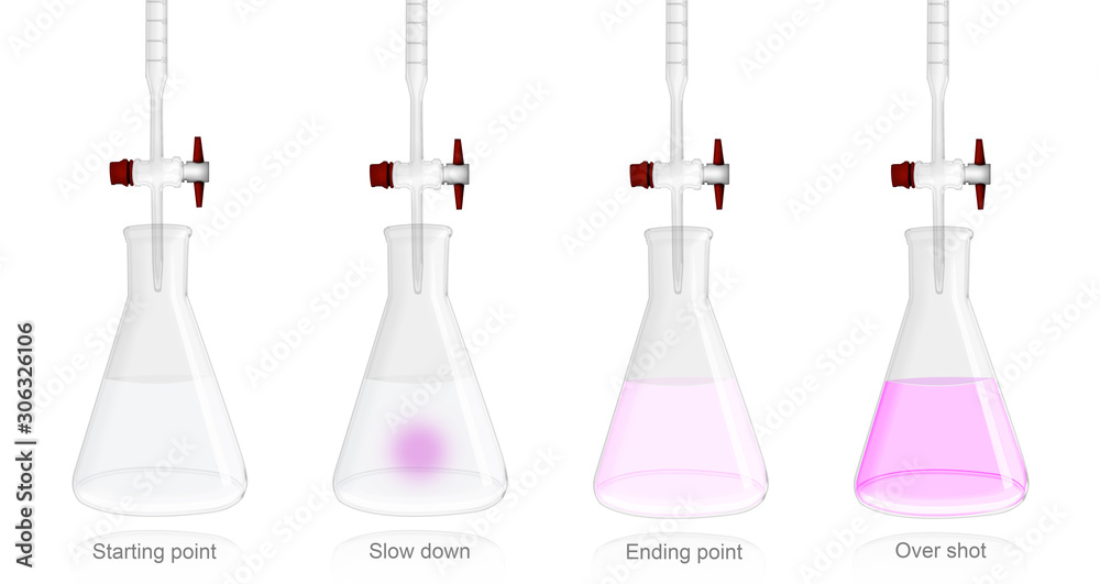
the endpoint of the titration is overshot manufacturer

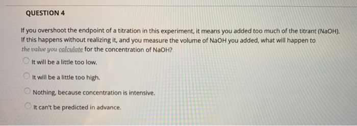
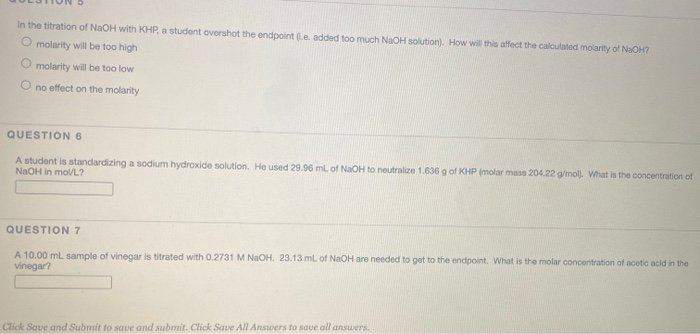
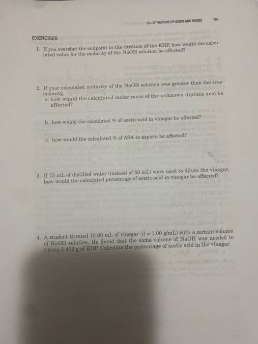
The endpoint of titration is overshot! Does this technique error result in an increase, a decrease, or have no effect on the reported percent acetic acid in the vinegar? Explain.

Titration is a quantitative analytical volumetric technique that permits the determination of the unknown concentration of an analyte with a known concentration of titrant. This is possible because the two react in a known stoichiometric manner allowing calculation of the unknown concentration.

This website is using a security service to protect itself from online attacks. The action you just performed triggered the security solution. There are several actions that could trigger this block including submitting a certain word or phrase, a SQL command or malformed data.

This website is using a security service to protect itself from online attacks. The action you just performed triggered the security solution. There are several actions that could trigger this block including submitting a certain word or phrase, a SQL command or malformed data.

A titration is a volumetric technique in which a solution of one reactant (the titrant) is added to a solution of a second reactant (the "analyte") until the equivalence point is reached. The equivalence point is the point at which titrant has been added in exactly the right quantity to react stoichiometrically with the analyten (when moles of titrant = moles of analyte). If either the titrant or analyte is colored, the equivalence point is evident from the disappearance of color as the reactants are consumed. Otherwise, an indicator may be added which has an "endpoint" (changes color) at the equivalence point, or the equivalence point may be determined from a titration curve. The amount of added titrant is determined from its concentration and volume:

A measured volume of the solution to be titrated, in this case, colorless aqueous acetic acid, CH3COOH(aq) is placed in a beaker. The colorless sodium hydroxide NaOH(aq), which is the titrant, is added carefully by means of a buret. The volume of titrant added can then be determined by reading the level of liquid in the buret before and after titration. This reading can usually be estimated to the nearest hundredth of a milliliter, so precise additions of titrant can be made rapidly.

Figure \(\PageIndex{1}\):The titration setup initially, before titrant (NaOH) has been added. NaOH is held in the burett, which is positioned above the beaker of acetic acid. Titrant (NaOH) is added until it neutralizes all of the analyte (acetic acid). This is called the equivalence point. Note: Unlike the picture, both substances are actually clear but are blue for visibility purposes in the picture.

As the first few milliliters of titrant flow into the flask, some indicator briefly changes to pink, but returns to colorless rapidly. This is due to a large excess of acetic acid. The limiting reagent NaOH is entirely consumed.

The added indicator changes to pink when the titration is complete, indicating that all of the aqueous acetic acid has been consumed by NaOH(aq). The reaction which occurs is

Reaction of acetic acid and sodium hydroxide to give acetate ion, sodium ion and water. The reaction is shown in terms of stick and ball diagram of each species.

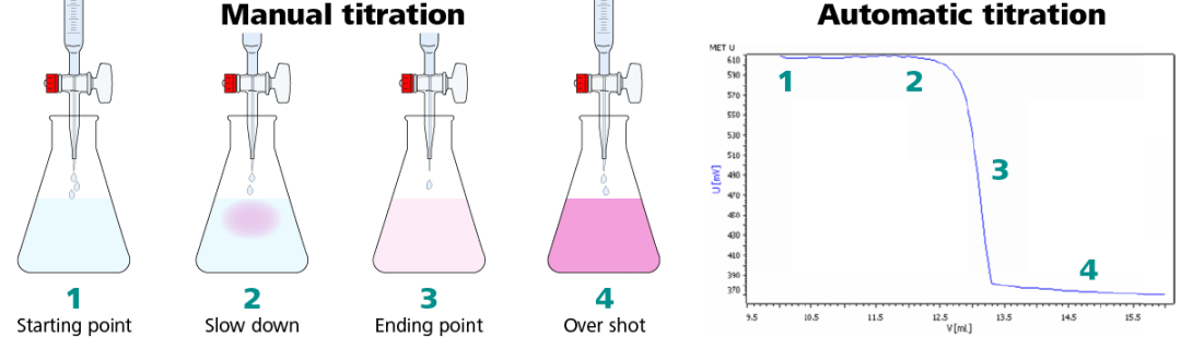
Eventually, all the acetic acid is consumed. Addition of even a fraction of a drop of titrant produces a lasting pink color due to unreacted NaOH in the flask. The color change that occurs at the endpoint of the indicator signals that all the acetic acid has been consumed, so we have reached the equivalence point of the titration. If slightly more NaOH solution were added, there would be an excess and the color of the solution in the flask would get much darker. The endpoint appears suddenly, and care must be taken not to overshoot the endpoint.

After the titration has reached the endpoint, a final volume is read from the buret. Using the initial and final reading, the volume added can be determined quite precisely:

Figure \(\PageIndex{2}\)The figure above shows a completed titration, where the equivalence point has been reached. NaOH (the titrant) has neutralized all of the Acetic Acid, leaving Acetate in the beaker. At this point, the moles of NaOH added is equivalent to the moles of acetic acid initially in the beaker.

The object of a titration is always to add just the amount of titrant needed to consume exactly the amount of substance being titrated. In the NaOH—CH3COOH reaction Eq. \(\ref{2}\), the equivalence point occurs when an equal molar amount of NaOH has been added from the graduated cylinder for every mole of CH3COOH originally in the titration flask. That is, at the equivalence point the ratio of the amount of NaOH, added to the amount of CH3COOH consumed must equal the stoichiometric ratio

Titration is often used to determine the concentration of a solution. In many cases it is not a simple matter to obtain a pure substance, weigh it accurately, and dissolve it in a volumetric flask as was done in Example 1 of Solution Concentrations. NaOH, for example, combines rapidly with H2O and CO2 from the air, and so even a freshly prepared sample of solid NaOH will not be pure. Its weight would change continuously as CO2(g) and H2O(g) were absorbed. Hydrogen chloride (HCl) is a gas at ordinary temperatures and pressures, making it very difficult to handle or weigh. Aqueous solutions of both of these substances must be standardized; that is, their concentrations must be determined by titration.

A sample of pure potassium hydrogen phthalate (KHC8H4O4) weighing 0.3421 g is dissolved in distilled water. Titration of the sample requires 27.03 ml NaOH(aq). The titration reaction is

To calculate concentration, we need to know the amount of NaOH and the volume of solution in which it is dissolved. The former quantity could be obtained via a stoichiometric ratio from the amount of KHC8H4O4, and that amount can be obtained from the mass

By far the most common use of titrations is in determining unknowns, that is, in determining the concentration or amount of substance in a sample about which we initially knew nothing. The next example involves an unknown that many persons encounter every day.

Vitamin C tablets contain ascorbic acid (C6H8O6) and a starch “filler” which holds them together. To determine how much vitamin C is present, a tablet can be dissolved in water andwith sodium hydroxide solution, NaOH(aq). The equation is

If titration of a dissolved vitamin C tablet requires 16.85 cm³ of 0.1038 M NaOH, how accurate is the claim on the label of the bottle that each tablet contains 300 mg of vitamin C?

The 308.0 mg obtained in this example is in reasonably close agreement with the manufacturer’s claim of 300 mg. The tablets are stamped out by machines, not weighed individually, and so some variation is expected.

This website is using a security service to protect itself from online attacks. The action you just performed triggered the security solution. There are several actions that could trigger this block including submitting a certain word or phrase, a SQL command or malformed data.

This invention relates to a system (method and apparatus) for the adjustment of electric potential of a liquid material to a predetermined aim by computercontrolled titration.

Titration is generally known as a method of determining volumetrically the concentration of a substance in a subject material by adding a standard solution of known volume and strength (this standard solution is known as the "titrant") to the subject material until a given reaction is completed.

Typically, titration is carried out to the "endpoint", i.e. the point at which the given reaction is complete, to determine the concentration of a given substance in the material. Various potentiometric, colorimetric, and coulometric titration processes are known in the art. Potentiometric determination methods are generally based on the determination of pH, ion activity, redox and other chemical potentials. Uses of titration techniques include determination of the contents of a chemical solution (See, U.S. Pat. No. 4,859,608 to Frueh) or to determine the concentration of certain functional chemical groups in a solution (See, U.S. Pat. No. 3,730,685 to Prohaska).

Titration processes require a high degree of precision, extensive operator interaction and are generally very time corisuining. Further, because the amount of titrant added to a solution to yield a given change will vary dramatically as the electric potential changes, overshooting the endpoint of a titration often occurs. Overshooting the endpoint of a titration results in inaccurate and often useless data or results.

In an effort to increase the accuracy and efficiency of titration processes, automatic titration systems have been developed. Most often these systems take the form of titration-to-endpoint methods mentioned above. In a typical endpoint system, the automatic titrator will produce a recording of the entire titration curve from which the endpoint may be determined.

In the curve-recording type of automatic system, titrant is delivered by means of a motor-driven syringe, or burette, through a capillary whose tip is immersed in a rapidly stirred solution. The motor drive is coupled to the drive mechanism of a recording potentiometer, with the recording chart divisions being directly related to the titrant delivered. The measured potential variations are automatically plotted on the chart, and by inspection of the plotted curve, the entrance and exit of the steep portion of the curve in which an inflection occurs can be located. By taking half the distance between these points, a close estimate of the endpoint is obtained.

One of the key advantages of an automatic titrator is that a large number of similar titrations can be performed in a short period of time, but the requirement for manual determination of the endpoint in each case obviates this advantage. In addition, poor results can occur if there is a slow attainment of equilibrium in the solution during the titration, or if the mixing rate is inadequate. This problem can be overcome to some extent by the use of an "anticipation" technique wherein the rate of titrant addition is automatically slowed as the end point is approached. However, anticipation does not entirely eliminate the problem, for the slower rate itself introduces errors and also reduces the advantage of the automatic system. It should also be noted that in many titrations, the points of inflection (areas of rapid change in electric potential that are indicative of the endpoint) on the plotted curve are very difficult to locate with any accuracy, and this introduces further error in the measurements.

There are many examples of automated titration-to-endpoint processes. U.S. Pat. No. 3,730,685 to Prohaska discloses a computer-controlled process whereby a program is used to analyze the progress of the titration curve by determining the slope of the curve after each incremental addition of titrant. The maximum slope of the curve is calculated to determine the endpoint of the titration.

U.S. Pat. No. 3,769,178 to Rethermal, Jr., discloses an automatic titration process that plots the first derivative of the titration curve in an attempt to more accurately determine the endpoint of the titration.

Other methods of automatic titration to determine the end point of the titration are disclosed in U.S. Pat. No. 4,266,942 to Vandenbossche et al., U.S. Pat. No. 4,302,299 to Ishikawa, and U.S. Pat. No. 4,859,608 to Frueh.

Titration processes may also be used to adjust the electric potential of a subject material. The adjustment may take the form of, for example, pH modification or the modification of the ion concentration in a material. U.S. Pat. No. 4,940,551 to Riggs et al. discloses a process where predetermined dispenses are injected into a fluid stream to create an in-situ titration curve to calculate one total dispense to obtain a desired pH. However, this system is slowed by the fact that the titration curve must be created before adjustment may commence.

The known processes utilizing automatic titration have been unable to completely solve such problems as excessive overshooting of the aim or endpoint, slow titration times or the requirement of operator interaction. Further, the known processes utilizing automatic titration are often restricted to pH applications or are designed for application only in titration-to-endpoint systems.

The present invention relates to a system (method and apparatus) for computer-controlled adjustment of the electric potential of a given material in liquid form. For the purposes of this invention, the electric potential to be adjusted may be in the form of a pH value, ion concentration (i.e., silver ion concentration measured in millivolts), redox or other chemical potentials. Controlled adjustment in accordance with the invention is to an "aim" which is not necessarily the endpoint but is a predetermined value of electric potential, which may correspond to a pH other than in the vicinity of a neutral pH (e.g. the aim for typical photographic emulsion of interest would be in the range of 4 to 7.5 pH units).

The method of the present invention utilizes a computer program to complete the electric potential adjustment of the material quickly and efficiently. The present process comprises two general phases: (a) a start-up phase, and (b) a final adjustment phase. The start-up phase is designed to calculate initial dispenses of titrant incrementally. The first initial dispense is calculated based on the slope number of other, previous titration curves of similar material.

The start-up phase is designed to use redispenses that are multiples of the first initial dispense until the electric potential is adjusted a desired minimum number of units toward the overall aim. This provides a minimum initial adjustment of the potential. After the minimum initial adjustment is made, the process proceeds to the final adjustment phase. Dispenses in the final adjustment phase may be calculated in one of two ways. If there were at least two dispenses during the start-up phase of the process, the next dispense will be calculated by fitting the data points to a mathematical equation and thereby extrapolating the volume of the next dispense. For example, the dispense may be calculated by application of a quadratic equation in which the measured electric potential is the principal parameter. However, if a mathematical expression cannot be established to fit through the data points that represent the previous dispenses (i.e., a positive real root of the quadratic expression for the fit not determined) then linear extrapolation must be used.

Therefore, if there has only been one dispense during the start-up phase, or there has been more than one dispense during the start-up phase but a mathematical expression cannot be fit relative to the data points, the dispense will be calculated by linear extrapolation.

In either case, the final adjustment phase of the process relies on the construction of a moving, in-situ titration curve that essentially plots the electric potential versus titrant volume and estimates future dispenses based on this curve.

To address the problem of overshoot, a sub-aim strategy is implemented in the final adjustment phase. The adjustments are made relative to these sub-aims, which approach the aim value. Additionally, the process is designed to terminate if certain events occur that decrease the accuracy of the adjustment.

The principal object of the present invention is to provide a system (method and apparatus) of computer-controlled adjustment of the electric potential of a quantity of material that is quick, efficient, exhibits a very small amount of aim overshoot and requires minimal operator interaction, which system is versatile and may be utilized to titrate materials of differing sensitivities to changes in titrant that may be known or unknown.

Referring to FIG. 2, shown is a diagrammatic illustration of one embodiment of an automatic titration system in accordance with present invention. The system of the present invention has wide-scale applicability to a variety of areas where adjustment by a method of potentiometric titration is useful such as pH adjustment, ion concentration adjustment or redox reaction processes. The present process has shown particular utility in the adjustment of pH and/or silver ion concentration of silver halide based photographic emulsions that are known in the art.

As shown in FIG. 2, titrant 102 is supplied from storage receptacle 104 (i.e., a beaker) by an automatic dispenser 110 which is commanded to produce dispenses (incremental volumes of the titrant) by an electrical compound signal which is outputted from a control computer 124 on electrical output line 112. Titrant 102 is pumped by a pump in dispenser 110 that is activated by the computer output.

Conduits 106 and 108 are tubes which carry the titrant. Fluid lines are shown solid and electrical lines are shown broken in FIG. 2. Receptacle 120 contains material 118 of which the electric potential is to be adjusted. The change in the electric potential is sensed by measurement probe 114 which is in contact with material 118 in receptacle 120. Measurement probe 114 is connected via line 116 to control computer 124 which digitizes the probe signal and contains the program which carries out the automatic titration method of the present invention.

Computer 124 may optionally include keyboard 126 for inputting data or other parameters, or a display 128 which may be a printer used to read out the titration results.

The program for the computer is shown for the exemplary case where adjustment of the electric potential of a photographic emulsion is of interest. Upon start, the program proceeds to store certain input parameters as shown at 2. These parameters include the initial meter reading, overall adjustment aim, batch size, titrant concentrations, minimum possible dispense volume and adjustment type (i.e., pH or silver ion concentration), the slope number and the titrant concentration (normality). Keyboard 126 may be used to input these parameters or they may be passed from other software programs integrated into computer 124.

As described above, the process of the present invention comprises two general phases: a start-up phase and a final adjustment phase. Additionally, the program has a system which tracks each dispense that is computed in the start-up and final adjustment phases. This system consists of the operations shown at 8 through 28.

The total number of dispenses during both the start-up and final adjustment phases is counted by operation 8. The electric potential is read as shown by operation 10. In this preferred embodiment, the electric potential is in the form of a pH or a value (in millivolts) representing the silver ion concentration of the material.

Next, decision 12 determines whether or not the reading is within the "aim tolerance". For purposes of this invention, the aim tolerance of an adjustment is the acceptable range of values on either side of the aim. The aim tolerance is an input which is stored upon initialization and may be set dependent on the needs and requirements of the individual adjustment being made. When the reading falls within the aim tolerance, the adjustment is stopped as indicated by terminal 14.

If the reading is not within aim tolerance, a decision 16 is made as to whether the aim has been overshot. If the aim has been overshot, the number of overshoots are counted by counting operation 18. If there have been more than two aim overshoots decision 20 recognizes that event and the adjustment procedure is stopped as indicated by terminal 22.

An integral part of the process of the present invention is the use of a sub-aim strategy. This enables the adjustments to be made rapidly without overshooting the desired aim value by using a series of sub-aims which approach the final aim value. This minimizes the chance of overshoots while maintaining aggressive movement toward the final adjusted aim.

Sub-aims may be determined in a variety of ways. In a preferred embodiment of the present process the sub-aims are determined from step tables. The step tables have two parts, one part is a sequence of steps (sub-aims) for approaching the overall aim and the other part is the range "in front of" each step to determine when the meter reading has been brought close enough to that step for the program to shoot for the next step. An exemplary pH step table used in a preferred embodiment of the process of the present invention is represented by Table I.TABLE I

Then the sub-aim is the difference between the If the reading is But not more than overall aim and greater than the the amount set forth the amount set amount set forth in in col. II from forth in col. III col. I from aim . . . aim . . . from aim I II III (pH units) (pH units) (pH units)

In another embodiment of the present process, the sub-aims may be set to change the electric potential by half the change needed to reach the aim (i.e. one-half the difference between the initial meter reading and the overall aim). The next sub-aim would be the overall aim value. This sub-aim method is used to approach the aim more aggressively when the possibility of overshoot is minimal, i.e. for adjustments where the slope of the titration curve is continuously decreasing. Additionally, a sub-aim may be established whereby the first sub-aim is the overall aim if the initial electric potential reading is within a predetermined number of units (pH units or millivolts) of the final aim.

After the program has looped through the tracking operations, the program branches as determined by decision 28 based upon the dispense count. When the count equals zero the start-up phase is entered. The dispenses calculated and made during the start-up phase ("initial dispenses") are calculated according to a predetermined start-up strategy. The start-up strategy may take any number of forms depending on the nature of the adjustment being made (i.e. pH or ion concentration), the data available, or the nature of the material being adjusted. The start-up strategy should be designed to make some minimal adjustment in the material before enough data has been obtained to use the more accurate methods of calculating dispense volumes that are embodied in the final adjustment phase. Additionally, the start-up strategy is designed to facilitate quick approach to the aim while minimizing the possibility of overshoot.

Exemplary start-up strategies may include a predictive component where equations are established that take into account certain parameters of the material being adjusted. These equations may be used to calculate initial dispenses that will give a desired initial adjustment. Another exemplary start-up strategy might involve the use of an initial bulk dispense of titrant to adjust the material by a relatively larger amount and calculate initial dispenses based upon the material"s response to the bulk addition.

A particularly preferred start-up strategy when adjusting silver halide based photographic emulsions is to calculate initial dispenses of titrant based on the slope number of a historical titration curve over a region of adjustment of the electric potential. The slope number represents an estimate of a titration curve slope over a region of adjustment of the material being adjusted. The titration curve from which the slope number is derived is based on batch history data from previous adjustments made on the same or similar material. The slope number quantifies the amount of titrant needed per unit change (i.e., pH units or millivolts) per unit mass of batch. The dispense volume is calculated at operation 30 using the slope number according to the following equation, denominated as Equation 1: ##EQU1## wherein Order=dispense volume (milliliters)

The extrapolation safety factor ("ESF") is implemented to prevent overshoots. This factor may be adjusted to cause the program to recommend some percentage of the full dispense calculated. The amount of the factor will vary depending on the type and nature of the adjustment. In this preferred embodiment, an ESF of 0.25 has been found particularly useful.

In a typical automatic titration system, dispenser 110 is capable of dispensing a minimum volume or more of titrant depending upon the command from computer 124 (FIG. 2). Therefore, after the initial dispense has been calculated in operation 30, the program compares the computed dispense volume with the minimum dispense volume (the minimum being stored upon initialization at operation 2) and decision 54 determines whether or not the dispense calculated is less than the minimum dispense volume of dispenser 110. If the initial dispense is below the minimum dispense, the sub-aim in effect is compared with the final aim at operation 56 to determine if the sub-aim for the adjustment equals the overall aim. If the sub-aim does not equal final aim the minimum volume (Dmin) is dispensed. If the sub-aim equals the overall aim, the process stops as shown at 58. If the calculated initial dispense (Dx) is not less than the minimum dispense (Dmin), the calculated initial dispense Dx is made as shown at 62.

At this point, the program provides time for equilibration of the electric potential as shown at 6. The program then returns to step 8 and the dispenses are counted. The electric potential is read at step 10. Decisions 12 and 16 are applied to determine if the electric potential is within aim tolerance or if the aim has been overshot. Next step 24 is carried out. There it is determined if the sub-aim has been achieved. If the sub-aim is achieved, the program will jump to the next sub-aim as shown at operation 26.

If decision 28 determines the dispense count does not equal zero then the total change in the electric potential (Δ) is computed at operation 36. If decision 38 determines that the original electric potential has been changed by less than a predetermined number of units, then the process will remain in the start-up phase for up to four more dispenses as shown at 48 (or until the minimum adjustment is attained). This continuation of the start-up phase provides flexibility when something has gone wrong with the adjustment (i.e., subject material buffered heavily, titrant or subject material concentrations erroneously determined, etc.)

The next dispenses ("redispenses") in the start-up phase ("DN ") are multiples of the initial dispense. Up to four redispenses of volume DN are computed in operation 52 based upon the initial dispense volume. The first redispense will be the same volume as the initial dispense. The second redispense will be two times the initial dispense. The third redispense will be three times the initial dispense and the fourth redispense will be four times the initial dispense. If the electric potential has not been adjusted the minimum amount after five dispenses as shown at 48, the adjustment will cease and the program terminates as shown at 50.

If the electric potential has been adjusted the minimum amount (K, as determined at decision 38), the start-up phase of the adjustment is complete. The program then proceeds into the final adjustment phase. In the final adjustment phase, the preferred method relies on the construction of a moving, in-situ titration curve that essentially plots the electric potential versus titrant volume for the last three data points and estimates future dispenses based on this curve. If less than three points of collected data exist, the curve will be based on whatever data has been compiled to that point.

Decision 40 determines if the dispense count is greater than one. If the dispense count is not greater than one, the first final dispense must be computed using a linear extrapolation of the response from the first initial dispense. The linear extrapolation is computed in operation 46 according to the following equation: ##EQU2## wherein Order=dispense volume (milliliters)=DLE

The linear extrapolation coefficient ("alpha") represents the fraction of the full dispense amount calculated by the linear extrapolation. Alpha is similar to the extrapolation safety factor discussed above. Alpha is a variable implemented to minimize the possibility of overshoots and may be dependent on a number of factors. In the embodiment presently described, for example, the type, range and direction of the adjustment were used to set alpha values. In general, it has been found that a higher alpha value may be used where the slope of the titration curve over the region of adjustment is decreasing because in that situation the chance of overshoot is less.

The calculated dispense DLE is treated as Dx as the program loops through operations 54, 56, 58, 60 and 62 and continues to loop through the control operations 12-28 and back, via connectors B--B, to compute the potential change Δ which determines whether further dispenses in the final adjustment phase are required.

If decision 40 determines that the dispense count is greater than one the program will attempt to extrapolate the next dispense volume by using a curve-fitting mathematical equation. The type of mathematical equation used is dependent on the type of adjustment and data obtained. For example, any number of polynomial equations, equations implementing natural logarithmic functions or equations implementing trigonometric functions may be used. In this embodiment of the method of the present invention, it has been found that extrapolation from a quadratic equation is particularly useful. In the present process, it is preferred to fit the quadratic through the last three data points and base the next dispense upon this curve. The quadratic extrapolation is carried out in operation 42 according to the following equation: ##EQU3## wherein .0.=zero

Next, test 44 will determine if the quadratic extrapolation has been successful and whether DQE is valid. If a positive real root is found, the quadratic extrapolation is successful and DQE is taken as valid and used as Dx in the same loop as used for DLE as discussed above. If a positive real root is not found then the next dispense is calculated by the linear extrapolation operation as shown at 46.

As with the start-up phase of the adjustment, all dispenses in the final adjustment phase go through decision 54 to determine if the calculated dispense is less than the minimum dispense volume of the dispensing means. If the dispense is less than the minimum dispense and the aim does not equal the overall sub-aim, the minimum volume is dispensed at 60. Otherwise, the volume calculated by either the quadratic extrapolation or the linear extrapolation is dispensed at 62.

Once the process is in the final adjustment phase, all remaining final dispenses are calculated utilizing the curve-fitting mathematical equation (i.e. quadratic extrapolation) if possible, in accordance with the above-described process, relative to the accessed sub-aims. The program will proceed from sub-aim to sub-aim until the electric potential has been adjusted to the predetermined, final aim.

Although the invention has been described in detail for the purpose of illustration, it is understood that such detail is for that purpose and variations can be made therein by those skilled in the art without departing from the spirit and scope of the invention. The foregoing description should therefore be taken as illustrative and not in a limiting sense.

In Table 1, the acid–base indicators are given, which are included in this paper. Their transition intervals, and the preparation of indicator solutions are included [12, 13]. All compounds were of analytical grade. To prepare the indicator Tashiro, Methylene blue from Riedel de Haën was used. The concentrations of the indicators were chosen so that the influence of the protonation/deprotonation of the indicator is negligible, but colours were clearly detectable.

o = 0.05 mol L−1, Merck) were used. Solid borax (disodium tetraborate decahydrate), Na2B4O7·10H2O (Merck), was used to prepare a stock solution with a concentration of 0.05 mol L−1. Titrations were performed by using standard glass burettes with a reading precision of 0.025 mL (half of a scale division). A certain amount of the sample was transferred with a standard glass pipette (±0.05 mL) into a conical flask, and it was filled up with water to about 100 mL. Then the indicator was added (resulting concentrations in the sample solutions are given in Table 1), and the titration was performed. Each experiment was repeated 10 times.

Sample solutions for potentiometric titrations were prepared in the same manner in a beaker. The titrant was added either with the standard glass burette in case of high concentrations of the sample, or with a transfer pipette (10–100 ± 0.6 μL, VWR, Germany) in case of small concentrations. Titrations were followed by using a glass electrode (InLab®, Mettler Toledo, Swiss) in conjunction with a pH metre 761 Calimatic (Knick, Germany). The glass electrode was calibrated before each measurement. For each sample and concentration, 11 experiments were performed (one with each indicator).

To construct the colour maps, the titration curves were recorded by measuring the pH of the solutions with a glass electrode, and the coloured solutions where photographed in spectrophotometric cuvettes. For this, Britton-Robinson buffer solutions were prepared according to [21] with a variation of the pH in 0.4 pH increments. For each indicator, these buffer solutions were prepared and the indicator was added in the concentrations given in Table 1. The pH of each buffer solution was measured in the absence and presence of the indicator, and no detectable differences could be noted. Individual pictures were taken and the colour maps were created using the freeware PhotoScape.

3 being an amino group. Additionally, the introduction of polar substituents, such as carboxyl or sulfonic acid groups increases the solubility of the compounds. Azo dyes are indicator bases. During protonation a cation is formed, and the positive charge is delocalized, i.e., resonance between the aromatic ring and a quinoide structure (Scheme 2). The colour change is from yellow to red (or red violet).

Schematic description of the structural changes of Azo dyes during protonation/deprotonation (only one resonance structure is given for the indicator base and two for the indicator acid)

Methyl orange is an orange powder. The sodium salt is moderately soluble in water. The aqueous stock solution should contain 0.1 % of the indicator. The transition interval is from 3.0 to 4.4 (Scheme 3).

o ≈ 5 × 10−4 mol L−1). The colours of the starting solutions (v = 0 and τ = 0 in Fig. 4) differ in case of high and low concentrations, because the titrations start at different pH values. In case of high concentrations, the starting colour is of vivid red pink (pH = 2.1), changing to red orange during progressive titration. At τ ≈ 0.91 (τ: degree of titration) the solution is already orange in colour (pH = 3.1). A distinct transition takes place between τ ≈ 0.985 and τ = (0.994 ± 0.002) from orange to bright yellow (pH ≈ 3.8–4.2, titration error at first bright yellow −0.6 %). In case of small concentrations the colour of the starting solutions is already orange (pH = 3.0). The transition from orange to bright yellow takes place between τ ≈ 0.8 and τ = (0.96 ± 0.01) (pH ≈ 3.7–4.4, titration error −4 %).

o ≈ 0.001 mol L−1) with 0.1 M NaOH and Methyl orange as indicator. Similar curves are observable for H2SO4. Dots experimental points, straight lines fits of experimental results with CurTiPot

o ≈ 5 × 10−3 mol L−1, pH = 2.4), the sample solution with Methyl orange is of vivid red pink, too (Fig. 5a). But the colour changes quickly to red orange during progressive titration. Already at τ ≈ 0.5 (pH = 3.8) the solution is yellow orange in colour. The transition takes place between τ ≈ 0.62 and τ = (0.90 ± 0.03) from yellow orange to bright yellow (pH ≈ 4.7, titration error −10 %). In case of low concentrations (C

o ≈ 5 × 10−4 mol L−1, pH = 3.3) the colour of the starting solution is already yellow orange (Fig. 5b). The transition from yellow orange to bright yellow is smeared out, and bright yellow is reached at τ = 0.83 ± 0.04 (pH ≥ 4.5, titration error −17 %).

o ≈ 5 × 10−4 mol L−1) with 0.1 M NaOH and Methyl orange as indicator. Dots experimental points, straight lines fits of experimental results with CurTiPot

o ≈ 5 × 10−4 mol L−1) are brilliant yellow before the addition of hydrochloric acid (pH = 9.2 and pH = 9.0 for high and low concentrations, respectively). In case of high concentrations, the transition from yellow to yellow orange (first orange undertone) is observable at τ = 1.012 ± 0.004 (pH = 4.3, titration error +1.2 %), but the colour changes gradually to orange, red orange and at least vivid red pink when continuing the addition of hydrochloric acid (i.e., large excess, pH < 3.0, cf. Figure 6a). In case of low concentrations, the transition from yellow to yellow orange is hardly visible at τ = 1.17 ± 0.06 (pH = 4.3, titration error +17 %), a real transition to orange and red orange is only obtainable, if an excess of hydrochloric acid is added (cf. Fig. 6b).

o ≈ 5 × 10−4 mol L−1) with 0.1 M HCl and Methyl orange as indicator. Dots experimental points, straight lines fits of experimental results with CurTiPot

Methyl red is a very common indicator for titrations of strong acids with strong bases. It is a dark red violet crystalline powder. In contrast to Methyl orange, it is sparingly soluble in water, and a stock solution should contain 0.02 % of the indicator in a 60 % ethanol water mixture. The transition interval is from pH 4.4 to 6.2 (Scheme 4). In the literature [13], the colour transition is given from yellow (base) to red (acid), but as it is shown in Fig. 7, a better description for the colour of the acid is fuchsia.

o ≈ 0.001 mol L−1) with 0.1 M NaOH and Methyl red as indicator. Similar curves are observable for H2SO4. Dots experimental points, straight lines fits of experimental results with CurTiPot

In case of high and low concentrations of strong acids, the sample solutions with Methyl red are of brilliant fuchsia colour (pH = 2.1 and pH = 3.0 for C

o ≈ 0.001 mol L−1, respectively). This colour does not change markedly during ongoing titration (Fig. 7a, b). The transition from fuchsia to yellow is very sharp. Only very close to the transition point (τ > 0.997 and τ > 0.98 in case of high and low concentrations, respectively, pH ≈ 4.5), the fuchsia colour starts getting lighter. At τ ≈ 1.000 (τ = 0.999 ± 0.002, high concentration, and τ = 1.00 ± 0.02, low concentration, pH ≈ 6–7) the complete solution is yellow. In both cases the systematic error is negligible, as we will discuss later in detail. However, it must be mentioned here, that the yellow colour vanishes with time, and the colour of the solutions returns to fuchsia because carbon dioxide from ambient air dissolves, and this decreases the pH of the solution. The rate of the regeneration of the fuchsia colour depends strongly on the experimental and ambient conditions, e.g. the return of the colour is very fast when the solution is heavily shaken. Hence, it is not serious to give a certain time span in which the colour should stay, although, this is often done in textbooks. In praxis, this leads very often to the fact that undergraduate students read the end point too late.

In case of a weaker acid like oxalic acid, the transition is not as sharp as for strong acids (cf. Fig. 8a, b). We can see here, that both solutions are fuchsia before titration starts. The brilliant fuchsia turns pale at τ > 0.90 (pH > 4.7). At τ ≈ 0.98 (pH = 5.5) the pale fuchsia turns to red orange, and the transition to clear yellow is obtained at τ = 0.990 ± 0.003 and τ = 0.99 ± 0.01 (pH = 5.7) for high and low concentrations of oxalic acid, respectively (titration error −1 %).

o ≈ 5 × 10−4 mol L−1) with 0.1 M NaOH and Methyl red as indicator. Dots experimental points, straight lines fits of experimental results with CurTiPot

In case of borax a sharp transition is observable; here the colour changes from yellow to brilliant fuchsia (Fig. 9a, b). At τ ≈ 0.99 (high concentration) and τ ≈ 0.98 (low concentration) (pH ≈ 6.0) the solutions start getting slightly orange (very weak orange undertone), and at τ = 1.000 ± 0.003 and τ = 1.00 ± 0.01 the transition to fuchsia for low and high concentrations is obtained, respectively (pH = 5.2). In both cases, the titration error is negligible.

To give sharper endpoint colour changes, Methyl red can be mixed with a dye insensitive to pH changes like Methylene blue (Scheme 5). This mixture is called Tashiro. The transition interval is that of Methyl red, the colour changes from violet (mixture of blue and brilliant fuchsia) to green (mixture of yellow and blue). At the transition point (pH = pK

Congo red, as the disodium salt, is a red powder. It is soluble in water, and the aqueous stock solution should contain 0.1 % of the indicator. The transition interval is from 3.0 to 5.0. This compound has a comparatively high salt error. It is a bisazo compound, resulting in a colour change different to that described above (cf. Scheme 6). In the literature [12], the colour transition is given from blue (acid) to red (base), but as shown in Fig. 11, it is better to describe the colour transition as blue violet to orange.

Sample solutions of high and low concentrations of hydrochloric acid and sulfuric acid with Congo red are pale blue violet (pH = 2.1 and pH = 3.0 for high and low concentrations, respectively, cf. Fig. 11a, b). In case of high concentrations the colour starts getting brighter already at τ ≈ 0.93 (pH ≈ 3.2). Between τ ≈ 0.98 and τ ≈ 0.99 (pH ≈ 3.7–4.0) the transition takes place from violet to red violet, and the solutions become orange above τ = 0.993 ± 0.002 (pH = 4.2, titration error −0.7 %). In case of low concentrations the transition from violet to red violet and at least to orange is observable between τ ≈ 0.8 and τ = (0.94 ± 0.02) (pH ≈ 3.7–4.3, titration error −6 %).

In case of oxalic acid, both titrations start with a pale blue violet colour (pH = 2.4 and pH = 3.3 for high and low concentration, respectively) (Fig. 12a, b). In case of high concentrations, at τ ≈ 0.7 (pH ≈ 3.8–4.0) it starts getting brighter and the solution becomes more violet. Between τ ≈ 0.80 and τ ≈ 0.85 the transition from red violet to orange red is observable, a clear orange is obtained at τ = 0.87 ± 0.02 (pH = 4.6, titration error −13 %). In case of low concentration, the transition interval is smeared out over a larger range of the titration degree; the solution starts getting brighter already about τ ≈ 0.5 (pH ≈ 3.8), and a clear orange is obtained already at τ = 0.77 ± 0.04 (pH = 4.5, titration error −23 %).

Figure 13a and b show the titration curves for high and low concentrations of borax with HCl and Congo red as indicator. In both cases, the solutions are orange before adding the HCl. In case of high concentration, the transition from orange via red violet to violet is rather sharp, it starts at τ ≈ 1.01 (pH = 4.5), and the transition to blue violet is obtained at τ = 1.014 ± 0.004 (pH = 4.0, titration error +1.4 %). In case of small concentration, the transition starts later at τ ≈ 1.05 (pH = 4.5), and the transition from red violet to blue violet is not as sharp as in case of high concentrations. A clear blue violet is obtained at τ = 1.15 ± 0.02 (pH = 4.0), i.e., the titration error is +15 %.

The Phthaleins (Scheme 7) are synthesised by heating phthalic anhydride with a derivative of phenol. All Phthaleins are rather insoluble in water but soluble in ethanol. In the acidic form most of the Phthaleins are colourless (lactone form), while in alkaline media a coloured quinoide structure is formed because of the opening of the lactone ring, i.e., most Phthaleins are monochromic indicators (Scheme 8).

Structural changes of Phthaleins during protonation/deprotonation (only one resonance structure is shown for the indicator acid and one resonance structure for the indicator base)

Structural changes of Phthaleins in strong alkaline solutions during protonation/deprotonation (pH > 13, only one resonance structure is shown for each species)

Phenolphthalein, one of the most popular indicators, can be considered as the basic compound of Phthaleins (Scheme 10). It is a white crystalline powder; stock solutions contain 0.05–0.1 % of the indicator in an ethanol water mixture of 50–70 % ethanol. The transition interval of phenolphthalein is from 8.0 to 10.

Solutions of high and low concentrations of strong acids as well as of weak acids appear colourless, when Phenolphthalein is added (see Figs. 14a, b, 15a, b). Under the conditions we consider here (concentration of Phenolphthalein is given in the experimental section, transition point at pH ≈ 8.5), for strong acids a sudden colour change to faint pink is obtained at τ = 1.003 ± 0.002 and τ = 1.02 ± 0.02 (high and low concentration, respectively). It is of outmost importance to avoid all colour influences from outside, meaning that the background is covered with white paper. The faint colour fades with time until the solution appears colourless again due to the influence of ambient air (cf. Methyl red). If the solution appears dark pink, the endpoint is overshot. Phenolphthalein is a suitable indicator for the titration of weak acids with a strong base as it can be seen in case of oxalic acid (Fig. 15a, b). Here, the colour turns to faint pink at τ = 1.000 ± 0.003 (high concentration) and τ = 1.01 ± 0.01 (low concentration).

o ≈ 5 × 10−4 mol L−1) with 0.1 M NaOH and Phenolphthalein as indicator. Similar curves are observable for HCl. Dots experimental points, straight lines fits of experimental results with CurTiPot

o ≈ 5 × 10−4 mol L−1) with 0.1 M NaOH and Phenolphthalein as indicator. Dots experimental points, straight lines fits of experimental results with CurTiPot

In contrast, Phenolphthalein is absolutely inappropriate as an indicator for the titration of weak bases with a strong acid, as it is depicted in Fig. 16a, b for borax. Although the sample solutions are pink, this colour fades quickly during ongoing titration, and the systematic deviation exceeds −40 % (τ = 0.54 ± 0.12 for high concentration, τ = 0.53 ± 0.08 for low concentrations).

o ≈ 5 × 10−4 mol L−1) with 0.1 M HCl and Phenolphthalein as indicator. Dots experimental points, straight lines fits of experimental results with CurTiPot

Thymolphthalein is a white crystalline powder; the structure is rather similar to Phenolphthalein with the exception that the two phenol groups are replaced by two thymol groups (Scheme 11). A stock solution contains 0.1 % of the indicator in an 80 % ethanol solution. Like phenolphthalein, it is a single-colour indicator. The transition range lies between pH 9.7 and 10.5.

Thymolphthalein turns from colourless to blue, but it has to be mentioned here, that it is only a fade blue, the transition is rather difficult to see and the influence of carbon dioxide from ambient air is rather pronounced due to the high pH values. In that range, the addition of about 5 × 10−5 mol L−1 of H3O+ ions leads to a change in pH of about 0.3 units. In case of strong acids (Fig. 17a, b), the first very faint blue colour is obtained between pH ≈ 9.7 and 10.0, i.e., τ = 1.009 ± 0.003 (high concentration, titration error +0.9 %), and τ = 1.06 ± 0.02 (low concentration, titration error +6 %). As in case of Phenolphthalein, it is important to avoid all colour influences from outside, and the progress of titration should be controlled with a white background.

o ≈ 0.001 mol L−1) with 0.1 M NaOH and Thymolphthalein as indicator. Similar curves are observable for H2SO4. Dots experimental points, straight lines fits of experimental results with CurTiPot

Similar results are obtainable with a weak acid like oxalic acid, as it is depicted in Fig. 18a, b. The first very faint blue colour is obtained between pH ≈ 9.7 and 10.0, i.e., τ = 1.006 ± 0.002 (titration error +0.6 %) in case of high concentration, and τ = 1.06 ± 0.02 (titration error +6 %) in case of low concentration.

o ≈ 5 × 10−4 mol L−1) with 0.1 M NaOH and Thymolphthalein as indicator. Dots experimental points, straight lines fits of experimental results with CurTiPot

Weak bases like borax are not titratable using Thymolphthalein as indicator. Here, already the sample solutions are colourless, as it is shown in Fig. 19a, b.

o ≈ 5 × 10−4 mol L−1) with 0.1 M HCl and Thymolphthalein as indicator. Dots experimental points, straight lines fits of experimental results with CurTiPot

Sulfonephthaleins (Scheme 12) are closely related to the Phthaleins and are formed by the reaction of o-sulfobenzoic acid anhydride with a phenol. They are sparingly soluble in water in the biprotonated form, whereas the monosodium salt is soluble in water. The structure contains the less stable sulfone ring which is opened already in acidic solutions. This leads to a quinoide structure, and the sulphonphthaleins are coloured in the acidic form, too. Sulfonephthaleins can be deprotonated in two steps [22]:

Bromophenol blue is an orange or light brown powder. Aqueous stock solution should contain 0.1 % of the monosodium salt of the indicator. The transition interval is from 3.0 to 4.6 (Scheme 14).

The solutions of high and low concentrations of hydrochloric acid and sulfuric acid with Bromophenol blue are pale yellow in colour (pH = 2.1 and pH = 3.0 in case of high and low concentrations, respectively, cf. Fig. 20a, b). In case of high concentrations, around τ = 0.97–0.98 (pH ≈ 3.5–3.7) the solutions start getting greenish yellow to grey and then to pale blue. The most striking colour change takes place at τ = 0.989 ± 0.003 (pH ≈ 4.0) the colour changes to blue purple resulting in a titration error of −1.1 %. During ongoing addition of the titrant, a smeared out colour change from blue purple to purple was observed. At lower concentrations, a faint greenish yellow colour is already visible at τ = 0.7 (pH ≈ 3.5), but the transition to blue purple takes place at τ = 0.94 ± 0.01 (pH ≈ 4.2), resulting in a titration error of −6 %.

o ≈ 5 × 10−4 mol L−1) with 0.1 M NaOH and Bromophenol blue as indicator. Dots experimental points, straight lines fits of experimental results with CurTiPot

In case of oxalic acid, the sample solution with high concentration of the acid (pH = 2.4) shows a pale yellow colour, too (Fig. 21a). Already at τ ≈ 0.6 (pH ≈ 3.6), the solution gets greenish yellow, and at τ ≈ 0.7 (pH ≈ 3.8–4.0) the colour changes via grey to pale blue. A clear transition to blue purple takes place at τ = 0.87 ± 0.02 (pH = 4.6), i.e., a titration error of −13 %. In case of low concentration of oxalic acid (Fig. 21b), the starting solution is greenish yellow in colour (pH = 3.3), and the colour changes slightly right from the beginning of the titration. Between τ ≈ 0.4 and τ ≈ 0.8, the colour turns gradually from pale blue to blue. The transition to blue purple takes place at τ = 0.86 ± 0.05 giving a titration error of −14 %.

o ≈ 5 × 10−4 mol L−1) with 0.1 M NaOH and Bromophenol blue as indicator. Dots experimental points, straight lines fits of experimental results with CurTiPot

Solutions of high and low concentrations of borax with Bromophenol blue as indicator are purple at the beginning, changing gradually to blue purple during ongoing titration (Fig. 22a, b). The blue colour starts degrading at τ ≈ 0.99 (high concentration) and τ ≈ 1.00 (small concentration) (pH ≈ 5.0–4.5). A transition from pale blue via grey to greenish yellow is observable between τ ≈ 1.00 and τ ≈ 1.03 for high concentrations, and between τ ≈ 1.01 and τ ≈ 1.15 for low concentrations, respectively (pH ≈ 4.5–3.2). If grey colour (pH ≈ 4.0) is taken for the determination of the transition point, the systematic errors are +1 and +8 % for high and low concentrations, respectively. In both cases, one will not end up with a clear pale yellow colour.

o ≈ 5 × 10−4 mol L−1) with 0.1 M HCl and Bromophenol blue as indicator. Dots experimental points, straight lines fits of experimental results with CurTiPot

Bromocresol green in the acidic form is a green powder. The monosodium salt is a dark red amorphous hydrate which becomes colourless at about 190 °C. The aqueous stock solution should contain 0.04 % of the indicator. The transition interval lies between pH 3.8 and 5.6 (Scheme 15).

Sample solutions with high concentrations of strong acids with Bromocresol green as indicator are yellow in colour (pH = 2.1, Fig. 23a). The colour changes at τ > 0.91 (pH > 3.1) to become greenish yellow, but a clear colour change from green to bright blue green is observed at τ = 0.999 ± 0.002 (pH ≈ 5.0, titration error −0.1 %), i.e., the systematic error is negligible. Also in case of small concentrations of strong acids, a sharp colour change is observed (Fig. 23b). The solutions are slightly greenish yellow right on from the beginning of the titration (pH = 3.0). Bright blue green solutions are observed for τ = 1.00 ± 0.01.

o ≈ 5 × 10−4 mol L−1) with 0.1 M NaOH and Bromocresol green as indicator. Dots experimental points, straight lines fits of experimental results with CurTiPot

A quite different result is obtainable in case of high and low concentrations of a weak acid like oxalic acid. Starting with a yellow solution, in case of high concentration (pH = 2.4) it becomes greenish yellow, soon; in case of low concentration we already start with a greenish yellow solution (pH = 3.3). The colour change is smeared out from turquoise to bright blue green between τ ≈ 0.70 and τ = (0.97 ± 0.01) (pH = 4.0–5.4) for high concentrations, and between τ ≈ 0.75 and τ = (0.91 ± 0.03) (pH = 4.4–5.0) for low concentrations (i.e., the titration errors are −3 and −9 %, cf. Fig. 24a, b).

o ≈ 5 × 10−4 mol L−1) with 0.1 M NaOH and Bromocresol green as indicator. Dots experimental points, straight lines fits of experimental results with CurTiPot

Solutions of borax in high and low concentration are bright blue green (pH = 9.2 and pH = 9.0 for high and low concentration, respectively), when Bromocresol green is added. Here, with ongoing addition of hydrochloric acid, the transition from blue green via turquoise to greenish yellow is rather sharp, and at τ = 1.009 ± 0.002 (high concentrations) and τ = 1.05 ± 0.02 (low concentrations) the greenish yellow colour is established (pH = 4.2, titration errors +0.9 and +5 %). In case of high concentrations, the colour will change until a yellow solution results, but this needs a markedly excess of hydrochloric acid (τ ≈ 1.1, pH ≈ 3.5). In case of small concentrations the solutions are still greenish yellow at τ ≈ 1.2 (pH ≈ 3.6) (cf. Fig. 25).

o ≈ 5 × 10−4 mol L−1) with 0.1 M HCl and Bromocresol green as indicator. Dots experimental points, straight lines fits of experimental results with CurTiPot

Thymol blue forms dark green crystals. A stock solution can be prepared by dissolving 100 mg of the indicator in a solution containing 0.001 mol L−1 sodium hydroxide. This indicator shows two transition regions: one at pH 1.2–2.8 from red orange to greenish yellow, and one at pH 8.0–9.6 from greenish yellow to blue (Scheme 16).

Only in case of high concentrations of strong acids, a smeared transition from red orange to greenish yellow can be observed at the beginning of the titration (cf. Fig. 26a), because the sample solutions have a pH = 2.1. In case of low concentrations of strong acids one already starts with a greenish yellow solution (pH = 3.0, cf. Fig. 26b). The same holds true for high and low concentrations of oxalic acid (pH = 2.4 and pH = 3.3, cf. Fig. 27a, b). In all cases, a sharp transition from greenish yellow to blue is obtained at the following degrees of titration: τ = 1.000 ± 0.003 (strong acid, high concentration), τ = 1.01 ± 0.02 (strong acid, low concentration), τ = 1.002 ± 0.003 (H2C2O4, high concentration), τ = 1.01 ± 0.01 (H2C2O4, low concentration), i.e., the titration error is negligible. But also here we can observe the influence of carbon dioxide (as it was already discussed in case of Methyl red). The blue colour turns quickly to green.

o ≈ 0.001 mol L−1) with 0.1 M NaOH and Thymol blue as indicator. Similar curves are observable for H2SO4. Dots experimental points, straight lines fits of experimental results with CurTiPot

o ≈ 5 × 10−4 mol L−1) with 0.1 M NaOH and Thymol blue as indicator. Dots experimental points, straight lines fits of experimental results with CurTiPot

In case of borax the sample solutions are blue, but the colour turns quickly to greenish yellow (τ ≈ 0.4), and a definite determination of a transition point is impossible (cf. Fig. 28a, b).

o ≈ 5 × 10−4 mol L−1) with 0.1 M HCl and Thymol blue as indicator. Dots experimental points, straight lines fits of experimental results with CurTiPot

Cresol red forms dark green–red crystalline powder. The stock solution should contain 0.04 % of the indicator. As in case of thymol blue, in very strong acidic solutions (pH < 1.8), the quinoide structure is protonated and the zwitter ion is red in colour. At pH values above 1.8, the deprotonated quinoide system is yellow, and the transition from yellow to vivid violet is between 7.2 and 8.8 (Scheme 17).

In all cases considered here, only the transition from yellow to vivid violet (or vice versa in case of borax) is considered. The transition is very sharp, very close to the transition point the solutions appears pale pink to nearly colourless (pH ≈ 7.3–7.8), (cf. Figs. 29a, b, 30a, b, 31a, b). As it was discussed already for other indicators, the influence of carbon dioxide from ambient air is very strong, during the titration of acids with a strong base. The colour turns quickly back to yellow. For all the three acids considered here in high and low concentration the titration error is negligible. The end points are obtained at the following degrees of titration: τ = 1.003 ± 0.003 (strong acid, high concentration), τ = 1.00 ± 0.01 (strong acid, low concentration); τ = 0.999 ± 0.002 (H2C2O4, high concentration), τ = 1.00 ± 0.02 (H2C2O4, low concentration).

o ≈ 5 × 10−4 mol L−1) with 0.1 M NaOH and Cresol red as indicator. Dots experimental points, straight lines fits of experimental results with CurTiPot

In case of borax we start with the vivid violet solutions (Fig. 31a, b). At τ ≈ 0.8 (pH ≈ 8.2) the colour turns to pale pink (nearly colourless). A clear transition from colourless to yellow is obtained at τ = 0.95 ± 0.01 (titration error −5 %) in case of high concentration and τ = 0.92 ± 0.02 (titration error −8 %) in case of low concentration (pH = 7.5).

Neutral red is one representative of other aromatic compounds suitable as acid base indicators. It is a dark green, nearly black powder moderately soluble in water and ethanol. Stock solutions contain 0.01 % of the indicator in an ethanol water mixture of 50–70 % ethanol. The transition interval ranges from 6.8 to 8.0. At pH values above 7.4, the uncharged molecule is the dominant species [24]. At lower pH values the cation is dominant (Scheme 18). The salt error of the compound is very small.

Structures of indicator acid and indicator base of Neutral red (only one resonance structure is displayed for the indicator base, two possible resonance structures are given for the indicator acid)

In case of strong and weak acids in both, high and low concentrations, the sample solutions are fuchsia, and a sharp transition from fuchsia via salmon to mustard yellow is observable (Figs. 32a, b, 33a, b), but solutions turn rapidly to fuchsia again under ambient conditions (see discussions above). For all the three acids considered here in high and low concentration the titration error is negligible. The end points are obtained at the following degrees of titration: τ = 1.001 ± 0.003 (strong acid, high concentration), τ = 1.00 ± 0.02 (strong, acid, low concentration); τ = 0.999 ± 0.002 (H2C2O4, high concentration), τ = 1.01 ± 0.02 (H2C2O4, low concentration).

o ≈ 5 × 10−4 mol L−1) with 0.1 M NaOH and neutral red as indicator. Similar curves are observable for HCl. Dots experimental points, straight lines fits of experimental results with CurTiPot

o ≈ 5 × 10−4 mol L−1) with 0.1 M NaOH and Neutral red as indicator. Dots: experimental points, straight lines: fits of experimental results with CurTiPot

In case of borax titrations, it is much more difficult to determine the end point, because the transition starts already at τ ≈ 0.95 (high concentration) and τ ≈ 0.90 (low concentration) (pH ≈ 7.5), and the colour changes from salmon via pale pink to fuchsia. A clear fuchsia is obtained at τ = 0.993 ± 0.004 (high concentration) and τ = 0.99 ± 0.02 (low concentration) (pH = 6.8, Fig. 34a, b).

o ≈ 5 × 10−4 mol L−1) with 0.1 M HCl and Neutral red as indicator. Dots experimental points, straight lines fits of experimental results with CurTiPot

Not sure what titration is or what you can do with it? Then you are in the right place! In this tutorial, you will find information on titration, including the chemicals that are commonly used and the chemical reactions that make titration work, as well as how titration is performed and some tips to get better results.

Titration is a method commonly used in chemistry to figure out the amount of a chemical in a solution. This chemical is called the titrand. To figure out the amount