mud pump discharge formula free sample

Rig pump output, normally in volume per stroke, of mud pumps on the rig is  one of important figures that we really need to know because we will use pump out put figures to calculate many parameters such as bottom up strokes,  wash out depth, tracking drilling fluid, etc. In this post, you will learn how to calculate pump out put for triplex pump and duplex pump in bothOilfield and Metric Unit.

Oil and Gas drilling process - Pupm output for Triplex and Duplex pumpsTriplex Pump Formula 1 PO, bbl/stk = 0.000243 x ( in) E.xample: Determine the pump output, bbl/stk, at 100% efficiency for a 7" by 12". triplex pump: PO @ 100%,= 0.000243 x 7 x12 PO @ 100% = 0.142884bbl/stk Adjust the pump output for 95% efficiency: Decimal equivalent = 95 + 100 = 0.95 PO @ 95% = 0.142884bbl/stk x 0.95 PO @ 95% = 0.13574bbl/stk Formula 2 PO, gpm = [3(D x 0.7854)S]0.00411 x SPM where D = liner diameter, in. S = stroke length, in. SPM = strokes per minute Determine the pump output, gpm, for a 7" by 12". triplex pump at 80 strokes per minute: PO, gpm = [3(7 x 0.7854) 1210.00411 x 80 PO, gpm = 1385.4456 x 0.00411 x 80 PO = 455.5 gpm

Example:Duplex Pump Formula 1 0.000324 x (liner diameter, in) x ( stroke lengh, in) = ________ bbl/stk -0.000162 x (rod diameter, in) x ( stroke lengh, in) = ________ bbl/stk Pump out put @ 100% eff = ________bbl/stk Example: Determine the output, bbl/stk, of a 5 1/2" by 14" duplex pump at 100% efficiency. Rod diameter = 2.0": 0.000324 x 5.5 x 14 = 0.137214bbl/stk -0.000162 x 2.0 x 14 = 0.009072bbl/stk Pump output @ 100% eff. = 0.128142bbl/stk Adjust pump output for 85% efficiency: Decimal equivalent = 85 100 = 0.85 PO@85%)= 0.128142bbl/stk x 0.85 PO@ 85% = 0.10892bbl/stk Formula 2

PO. bbl/stk = 0.000162 x S[2(D) - d] where S = stroke length, in. D = liner diameter, in. d = rod diameter, in. Example: Determine the output, bbl/stk, of a 5 1/2". by 14". duplex pump @ 100% efficiency. Rod diameter = 2.0in.: PO@100%=0.000162 x 14 x [ 2 (5.5) - 2 ] PO @ 100%)= 0.000162 x 14 x 56.5 PO@ 100%)= 0.128142bbl/stk Adjust pump output for 85% efficiency: PO@85%,= 0.128142bb/stkx 0.85 PO@8.5%= 0.10892bbl/stk Metric calculation Pump output, liter/min = pump output. liter/stk x pump speed, spm. S.I. units calculation Pump output, m/min = pump output, liter/stk x pump speed, spm. Mud Pumps Mud pumps drive the mud around the drilling system. Depending on liner size availability they can be set up to provide high pressure and low flow rate, or low pressure and high flow rate. Analysis of the application and running the Drill Bits hydraulics program will indicate which liners to recommend. Finding the specification of the mud pumps allows flow rate to be calculated from pump stroke rate, SPM. Information requiredo Pump manufacturer o Number of pumps o Liner size and gallons per revolution Weight As a drill bit cutting structure wears more weight will be required to achieve the same RoP in a homogenous formation. PDC wear flats, worn inserts and worn milled tooth teeth will make the bit drill less efficiently. Increase weight in increments of 2,000lbs approx. In general, weight should be applied before excessive rotary speed so that the cutting structure maintains a significant depth of cut to stabilise the bit and prevent whirl. If downhole weight measurements are available they can be used in combination with surface measurements to gain a more accurate representation of what is happening in the well bore.

Whether you operate an industrial pump or looking to purchase the right pumps in India for your needs, the flow rate of the system is a crucial parameter. In this guide, Sintech, the no.1 industrial

Flow rate is the amount of fluid that the pump can transport within a given time. Knowing the flow rate of your pump can help you achieve two key things:

You can figure out if your system is working efficiently. If you know the expected flow rate and the current flow rate, then you can identify if your system is underperforming. This helps you make the right action to improve the pump’s performance.

Before you approach multistage centrifugal pump manufacturers in India for your purchase needs, having an idea of the desired flow rate will help you plan the system design perfectly. If you calculate the required flow rate wrong, then you would install an oversized/undersized pump, which is not a good investment in the long run. So, you need to have a clear idea of the desired flow rate before ordering the best pumps in India from your preferred manufacturer.

You need to calculate three factors before ordering the right pumps:The type of fluid you need to pump – is it viscous or clear? What’s the temperature of the pumped fluid? Etc.

The volume of fluid that needs to be transported in a specific timeAll these three factors will vary based on your industrial needs. The volume of fluid that you want to transport determines the flow rate of the pump. The type of fluid and the distance transported both play a huge role in impacting the flow rate that you can achieve. Hence, all these three factors play a crucial role in determining the size and type of pump needed.

We highly recommend that you contact a pump sizing expert to help you decide the correct equipment to buy. At Sintech, we offer free pump sizing guidance for all our clients, to help them find the best pumps in India for their requirements.

Once you have installed the pump, you need to monitor the flow rate periodically to determine if your pump is performing efficiently. You can check the pump’s performance by monitoring several factors. Right now, we’ll just calculate the flow rate.

You can measure the flow rate of an operating pump using either one of the following two methods:Use a flow meter – A flow meter is a simple device that does exactly what it means – it measures the amount of fluid passing through the system. Attach the flow meter to the discharge outlet. The reading on the meter gives you the flow rate of the system.

Calculate flow rate manually by collecting fluid – You can collect the fluid at the output of the pump system using a bucket or vat. Measure the collected fluid, the time taken to collect it, and reverse engineer to find the flow rate. The formula for calculating the flow rate: Flow rate = Volume of Liquid Collected / Time Taken

If there is a significant difference between desired flow rate and the actual flow rate, you can then carry on an inspection of the pump system to determine what’s wrong. Or if it’s time for a pump replacement, then Sintech Pumps, the no.1 multistage centrifugal pump manufacturers in India has an excellent range of industrial pumps for all needs. Get in touch with our team to find the right pumps for your specific needs.

Pumps tend to be one of the biggest energy consumers in industrial operations. Pump motors, specifically, require a lot of energy. For instance, a 2500 HP triplex pump used for frac jobs can consume almost 2000 kW of power, meaning a full day of fracking can cost several thousand dollars in energy costs alone!

So, naturally, operators should want to maximize energy efficiency to get the most for their money. Even a 1% improvement in efficiency can decrease annual pumping costs by tens of thousands of dollars. The payoff is worth the effort. And if you want to remotely control your pumps, you want to keep efficiency in mind.

In this post, we’ll point you in the right direction and discuss all things related to pump efficiency. We’ll conclude with several tips for how you can maintain pumping efficiency and keep your energy costs down as much as possible.

In simple terms, pump efficiency refers to the ratio of power out to power in. It’s the mechanical power input at the pump shaft, measured in horsepower (HP), compared to the hydraulic power of the liquid output, also measured in HP. For instance, if a pump requires 1000 HP to operate and produces 800 HP of hydraulic power, it would have an efficiency of 80%.

Remember: pumps have to be driven by something, i.e., an electric or diesel motor. True pump system efficiency needs to factor in the efficiency of both the motor AND the pump.

Consequently, we need to think about how electrical power (when using electric motors) or heat power (when using combustion engines) converts into liquid power to really understand pump efficiency.

Good pump efficiency depends, of course, on pump type and size. High-quality pumps that are well-maintained can achieve efficiencies of 90% or higher, while smaller pumps tend to be less efficient. In general, if you take good care of your pumps, you should be able to achieve 70-90% pump efficiency.

Now that we have a better understanding of the pump efficiency metric, let’s talk about how to calculate it. The mechanical power of the pump, or the input power, is a property of the pump itself and will be documented during the pump setup. The output power, or hydraulic power, is calculated as the liquid flow rate multiplied by the "total head" of the system.

IMPORTANT: to calculate true head, you also need to factor in the work the pump does to move fluid from the source. For example, if the source water is below the pump, you need to account for the extra work the pump puts in to draw source water upwards.

*Note - this calculation assumes the pump inlet is not pressurized and that friction losses are minimal. If the pump experiences a non-zero suction pressure, or if there is significant friction caused by the distance or material of the pipe, these should be factored in as well.

You"ll notice that the elevation head is minimal compared to the discharge pressure, and has minimal effect on the efficiency of the pump. As the elevation change increases or the discharge pressure decreases, however, elevation change will have a greater impact on total head.

Obviously, that’s a fair amount of math to get at the pump efficiency, considering all of the units conversions that need to be done. To avoid doing these calculations manually, feel free to use our simple pump efficiency calculator.

Our calculations use static variables (pump-rated horsepower and water source elevation) and dynamic variables (discharge flow and pressure). To determine pump efficiency, we need to measure the static variables only once, unless they change.

If you want to measure the true efficiency of your pump, taking energy consumption into account, you could add an electrical meter. Your meter should consist of a current transducer and voltage monitor (if using DC) for electrical motors or a fuel gauge for combustion. This would give you a true understanding of how pump efficiency affects energy consumption, and ultimately your bank account.

Up until this point, we’ve covered the ins and outs of how to determine pump efficiency. We’re now ready for the exciting stuff - how to improve pump efficiency!

One of the easiest ways to improve pump efficiency is to actually monitor pumps for signs of efficiency loss! If you monitor flow rate and discharge (output power) along with motor current or fuel consumption, you’ll notice efficiency losses as soon as they occur. Simply having pump efficiency information on hand empowers you to take action.

Another way to increase efficiency is to keep pumps well-maintained. Efficiency losses mostly come from mechanical defects in pumps, e.g., friction, leakages, and component failures. You can mitigate these issues through regular maintenance that keeps parts in working order and reveals impending failures. Of course, if you are continuously monitoring your pumps for efficiency drops, you’ll know exactly when maintenance is due.

You can also improve pump efficiency by keeping pumps lubricated at all times. Lubrication is the enemy of friction, which is the enemy of efficiency (“the enemy of my enemy is my friend…”).

A fourth way to enhance pump efficiency is to ensure your pumps and piping are sized properly for your infrastructure. Although we’re bringing this up last, it’s really the first step in any pumping operation. If your pumps and piping don’t match, no amount of lubricant or maintenance will help.

In this post, we’ve given you the full rundown when it comes to calculating and improving pump efficiency. You can now calculate, measure, and improve pump efficiency, potentially saving your business thousands of dollars annually on energy costs.

For those just getting started with pump optimization, we offer purpose-built, prepackaged solutions that will have you monitoring pump efficiency in minutes, even in hazardous environments.

Discharge Head: This is the vertical distance that you are able to pump liquid. For example, if your pump is rated for a maximum head of 18 feet, this does not mean that you are restricted to 18 feet of pipe. You can use 300 feet, so long as the final discharge point is not higher than 18 feet above the liquid being pumped.

Suction Lift: This is the vertical distance that the pump can be above the liquid source. Typically, atmospheric pressure limits vertical suction lift of pumps to 25 feet at sea level. This does not mean that you are limited to 25 feet of pipe. You could use upwards of 300 feet of suction pipe, so long as the liquid source is not lower than 25 feet below the pump center line.

Pumps are an integral part of almost all industries today. From construction and mining to automotive and aerospace, pumps play a vital role in keeping these industries moving forward. While there are many essential parameters in pumps, one critical parameter is the pump flow rate which becomes a guiding factor for pump manufacturers.

The pump flow rate is one of the most important factors to consider when selecting a pump. It measures how much water the pump can move in a given period of time and is typically expressed in cubic meters/hour (m3/ h). If you’re looking for a pump to use in your home or business, it’s essential to know the flow rate needed to meet your needs. Otherwise, you may end up with a pump that isn’t powerful enough or one that uses more energy than necessary.

The first step is to determine what your needs are. For example, if you’re using the pump to provide water for irrigation, you’ll need to know the maximum flow rate that will be required. Once you know your needs, you can start looking for pumps that have the required flow rate, as you will now be able to give more precise directions to the pump manufacturers about your requirement.

To choose the right pump, it’s also important to consider other factors, such as pump size and efficiency. For instance, a large pump with a high flow rate may be more expensive to purchase and operate than a smaller pump with a lower flow rate. However, it may still be the better option if your water usage is consistently high or you have multiple zones in your irrigation system that need water simultaneously.

Overall, choosing the right pump for your home or business requires careful consideration of all aspects of pumping performance. With the right pump from reliable pump manufacturers, you can rest assured that you’ll always have an adequate supply of water on demand.

Pump flow rate simply refers to the volume of fluid that is moving through a pump in a given time period. There are various units through which it is measured, and they include cubic meter/hour (m3/h), litre/sec (l/s) or gallons per minute (GPM). Different pump manufacturers refer to different pump flow units.

The flow rate of a pump can be affected by several factors, including the size and type of pump, the speed at which it is operating, and the resistance of the system it is pumping into.

Pump Speed: This is the number of times the pump can complete an entire cycle in a minute and is measured in rotations per minute (rpm). The faster the pump speed, the higher the flow rate.

Pump Size: Larger pumps can move more liquid than smaller pumps. This is why it’s essential to choose an appropriately sized pump for your application.

Now that you know the basics of pump flow rate, you can begin to select a pump that is appropriate for your application. Keep in mind that the factors listed above will all affect pump flow rate, so it’s essential to consider each one when you give your requirements to the pump manufacturers.

Pump speed is measured in revolutions per minute (rpm). To convert from rpm to hertz, divide by 60. For example, if a pump operates at 1000 rpm, its frequency would be 16.67 Hz.

Let’s say you have a pump that is operating at 1000 rpm, has an impeller size of 6 inches, and is pumping water with a density of 62.4 lb/ft3. So the flow rate would be:

There are a few key ways to increase the flow rate efficiency in pumps. One is to choose the right pump for the application. Another way is to ensure that the pump is sized correctly for the application. Additionally, regular maintenance can help keep a pump operating at peak efficiency.

When choosing a pump, it is vital to consider the application’s specific needs. For example, if a pump is handling a corrosive fluid, you should select stainless steel or other corrosion-resistant models. Similarly, if the fluid being pumped will be unusually viscous, then a positive displacement pump may be the best option.

Ensuring that a pump is appropriately sized for its application is also critical to maximizing flow rate efficiency. If a pump is too small for the task at hand, it will have to work much harder and will be less efficient. On the other hand, if a pump is too large for the application, it will not operate at peak efficiency.

Finally, regular maintenance is essential to keeping a pump operating at its best. This includes things like inspecting and cleaning the pump regularly and making sure that all of the moving parts are adequately lubricated. By taking these steps, it is possible to keep a pump running at peak efficiency for many years.

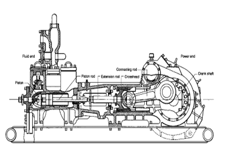
Since the NOV A1700-PT Triplex Mud Pump was built approximately 60 years ago, the industry has widely accepted the three cylinder or triplex style pump. Triplex mud pumps are manufactured worldwide, and many companies have emulated the original design and developed an improved form of the triplex pump in the past decade.

NOV A1700-PT Triplex Mud Pumps have many advantages they weight 30% less than a duplex of equal horsepower or kilowatts. The lighter weight parts are easier to handle and therefore easier to maintain. The other advantages include;They cost less to operate

One of the more important advantages of triplex over duplex pumps, is that they can move large volumes of mud at the higher pressure is required for modern deep hole drilling.

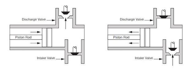
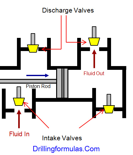
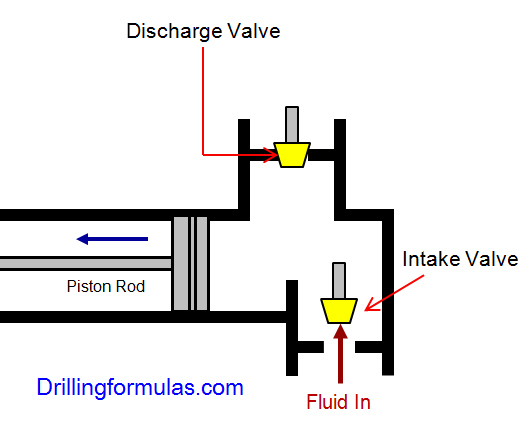
NOV A1700-PT Triplex Mud Pump is gradually phasing out duplex units. In a triplex pump, the pistons discharge mud only when they move forward in the liner. Then, when they moved back they draw in mud on the same side of the piston. Because of this, they are also called “single acting.” Single acting triplex pumps, pump mud at a relatively high speeds. NOV A1700-PT Triplex Mud Pump has three pistons each moving in its own liner. It also has three intake valves and three discharge valves. It also has a pulsation dampener in the discharge line.

The “pond” is actually a man made dam which covers an area of about 40ha and has rockfill embankments of up to 53m high along the southern side that forms the impoundment.  It initially constructed in 1959 to act as a tailings pond to take the bauxite residue (red mud) from the Ewarton Plant situated about 5km away and 300m lower.  The red mud was pumped as a slurry comprising about 20% solids to the pond over a period of about 32 years up to 1991 when the pond was replaced by the Charlemount Mud Stacking and Drying Facility.  During this period the pond embankments (referred to as dams), were raised up to 7 times providing a final crest elevation of 472m.  The pond was however never filled to its final design capacity and the mud beach level remained at about 469m and the central area about 458m leaving a concave depression which held about 1.4mil m3 of water with elevated pH and some caustic content.

The remediation plan for the pond includes the removal of the ponded water and then the regrading of the mud surface to be free draining so that it can be stabilised and vegetated.  About 500,000 m3 of mud will need to be moved over a distance of up to 1km in order to create the required profile.  Due to the very soft nature of the surface muds (shear strength of less than 3kPa) its bearing capacity is less than 20kPa hence it is not accessible using even modified earthworks equipment.  In addition, the muds are thyrotrophic and under any vibration or shear loading, rapidly liquefy resulting in significant reduction in shear strength and loss of bearing capacity.  Using conventional earthmoving equipment would therefore require extensive “floating” haul roads with a high risk of machinery getting stuck or entire plant loss and risk to personnel.  It was therefore decided to investigate the possibility of pumping the in-situ red mud.

A mud pumping trial was undertaken to assess the feasibility of using this technique to do the bulk mud moving.  Pumping red mud is not unusual and the muds were initially pumped up to Mt Rosser Pond.  However, the muds are usually pumped at a solids content of 30% or less.  Once deposited, they can take years to reconsolidate and firm up sufficiently to allow access for light earthworks and agricultural plant.

In addition to the mud pumping, the trial included infilling three small scale geotubes to assess their performance as these may be needed as part of the regrading works.

The main aim of the pump trial was to determine if the muds could be pumped in their insitu state, and if not, what amount of water is required and how the variations in water content affect pump rates.

The mud pumping trial was undertaken using a 4” EDDY Pump.  This pump was recommended due to its ability to handle variable solids and robust operating mechanism.  The pump unit incorporated a hydraulic drive and cutter head.  The unit was mounted onto the boom of a JCB 220 excavator which also supplied the hydraulic feed to power the pump for the required range of 30-40 GPM at 3,500 to 4,000 psi (2428MPa).  The cutter head was powered by a standalone hydraulic power unit capable of providing the required 30gpm at 200psi (1.9 l/s at 13.8MPa).  If mounted on a 30-ton excavator with a System 14 hydraulic system and dual auxiliary feeds to the boom, all necessary hydraulic power for the pump and cutter head can be supplied by the excavator.  This equipment was however not available at the time in Jamaica.

In addition to the pump mounted on the excavator a Long Reach excavator (CAT 325) was used to move muds towards the cutter head but also to loosen up the muds and mix in additional water to facilitate pumping.  Water was added by pumping it directly from the pond using a 3” diesel water pump.

Prior to pumping the muds, the mud pump would operate in recirculation mode in order to prime the pump.  When in recirculation (re-circ) mode, the material pumped would be diverted to a short discharge pipe mounted on the pump directed back parallel to the cutter head. This action would help agitate and stir the muds.

A geotechnical soils investigation was undertaken on the muds within Mt Rosser pond in 2004.  It showed the material to be predominantly clayey silt with approximately 13% sand, 29% clay and 58% silt using conventional sieve analysis and hydrometer.  Atterberg limits indicate that the material is an intermediate to high plasticity clay.  The muds do however vary across the lake and also vertically. This is mainly as a consequence of the deposition process and discharge location.  Close to the discharge location the courser materials would settle out first and the finer materials would disperse furthest and to the opposite end of the pond.  The results are presented in figure 4.1.

Earlier this year, additional mud samples were tested as it was evident that standard soil mechanics tests did not provide an accurate assessment of this fine material.  This was particularly evident in tests done with dry sieving which shows the material as well-graded sand (see results for samples 5300, 5301, 5302 on figure 4.2).  When dispersed in water, even with an agent, the ‘yield-pseudo-plastic’ rheology of the muds appeared to affect the hydrometer results with large variations between tests (see results of samples PFT4&5 taken during mud pumping trials on figure 4.2).

The additional testing comprised of undertaking gradings using a Laser Particle Analyzer. The results indicated that the muds are predominantly Silt although the silt % varied from 30% to 80% with the material being either more sandy or more clayey (up to 15% clay). See results of samples ending in “L” on figure 4.2 below.

Moisture content tests on the muds taken from within the mud pond but below the ponded water ranged from 100% to 150% (50% to 40% solids).  The muds at the pump test location were 137% (42% solids).

Shear strength was generally very low ranging from 1kPa to 6kPa increasing with depth.  Dynamic probes previously undertaken indicated that the muds are “very soft” to 5m increasing in strength slightly to “soft” at a depth of 9m after which they increase to firm becoming stiff.

The pH of the muds ranged from 10.3 to 11.7, (ave 11.2).  Previous testing indicated that the surface muds have the lower pH although once through the crust, the pH tends to be higher. When doing the trials, the muds up to a depth of about 2.5m was intermixed, hence any stratification in pH could not be determined.

Initially, pumping was problematic mainly due to the excavator being underpowered. This was diagnosed as a hydraulic pump problem and the excavator was replaced.  The cutter head (which also acts to protect the intake) tended to blind with mud (Photo 5.1) and was also not providing enough agitation to liquefy the muds.  This was partly resolved by adding “stirrers” (2 steel loops welded either side) to the rotating cutter head and also a “comb” (Photo 5.2) to keep the gaps within the cutter head open.

Mud pumping rates varied from 21 l/s to 52 l/s (332 – 824gpm) and it was clearly visible that the more liquid the muds were the higher the pump rate was.  Samples were taken at different discharge rates and moisture content and percent solids determined by laboratory testing.  The results are plotted in Figure 5.1 and although scattered, do give an indication of the effects of solids content on flow rates.  The natural moisture content of the muds (insitu) at the test location was 137%, or 42% solids.  This is shown in Figure 5.1 as a vertical line.  Pumping muds close to the percent solids was achieved although flow rates were low.

As mentioned previously, the long reach excavator was used to loosen up the muds.  Water was pumped from the pond using a 3” pump into the excavation and the long reach would then work the muds to mix the water in.  The mud pump would then be used in recirculation mode to further mix the muds into a more consistent state.  Even with this mixing and agitation, the water tended to concentrate on the surface. This aided the initial process of priming the pump and once primed thicker muds at 1m to 2m below the surface could be pumped.  However, it was found that the deeper muds tended to be lumpy and this would significantly reduce or stop the flow requiring the pump to be lifted into thinner muds or having to go back into re-circ mode or having to fully re-prime.  The pump discharge was therefore very inconsistent as the suction intake position constantly needed adjustment in an attempt to get adequate discharge but also pump the thickest muds possible.

Discharge of the pumped muds was through 30m of flexible hose then 60m of 4” HDPE pipe which had an internal diameter of about 87mm (3.5”).    The muds were discharged onto the original mud beach which lies at a gradient of about 9%. On deposition the muds slowly flowed down gradient.  At times the flow would stop and the muds would build up then flow again in a wave motion.  The natural angle of repose would therefore be a few degrees less than this – probably 5% to 6%.

Although the muds have very low shear strength, and on agitation liquefy, the sides of the excavation had sufficient strength to stand about 2m near vertical.  Even overnight, there was limited slumping and the bank could be undermined by about 0.5m with the cutter head/agitator before collapsing.

On termination of pumping, in order to flush the pipeline, thin watery muds were pumped until the line was clear. A “T” valve system was then used to connect the 3” water pump line and this was then used to flush the pipe with water.

Three geotubes (1m x 6m) were filled with red muds pumped using the 4” Eddy pump. Fill rates were about 30 to 40l/s although it was difficult to assess as the flow and mud consistence was not visible.

Tube 1 was filled initially with more runny mud and then thicker muds as the pump operator got a better feel for conditions.  The tube was filled until firm.  The second tube was filled with thicker muds and filling continued until the tube was taut.  These two tubes were positioned on the sloping beach in order to form a small “U” impoundment area that would later be filled with pumped muds.  Although the area was prepared, the sloping ground caused the first tube to rotate through about 20 degrees. The tube was staked and the downslope side backfilled.  A more defined bed was created for the second tube and the same rotational issue was limited.  The two filled tubes with the ponded mud are shown in Photos 5.7 and 5.8.  Other than a small leak at the contact between the two geotubes, the ponding of the muds was successful.

The third tube was positioned on level ground. It was filled with medium runny (but consistent thickness) muds and was filled until the tube was taut.

In all three cases, there was very little mud loss or seepage from the tubes.  When stood on, some red water would squeeze out around the pressure area.  Once filled taut, the entire bag would have small red water droplets form on the outside (visible in Photo 5.11) , but the seepage was in general nominal.

The tubes have been monitored and the most recent photo’s taken on 10 October 2011 (6 weeks after filling) show how the tubes have reduced in volume due to the dewatering of the contained muds.  Volume loss is estimated to be around 30%.  The anticipated moisture content would therefore be about 90% and the solids around 53%.

The muds pumped into the trial pond behind the geotubes were medium thick to thick, probably in the order of 37 – 40% solids.  After 6 weeks the mud has not only firmed-up but had dried out significantly with wide and deep surface cracks as are evident in Photo 5.14 and 5.15.

The muds can be pumped at close to their insitu moisture content and most likely at their in-situ moisture content if they were agitated more and the pipeline system was designed to reduce friction losses.

Be able to access the mud surface and move around efficiently and safely. The suggestion is to have the pump mounted on a pontoon that is positioned using high strength rope (dynema) or steel cable.  The pump system should be remotely controlled as this would limit regular movement of personnel on the muds.

Have sufficient power and volume capacity to pump the muds at close to or at in-situ moisture content and discharge them about 1000m through a flexible pipeline.

It was also evident from the trials that the muds do not slump and flow readily.  It will therefore be necessary to have an amphibious excavator to loosen up the muds in the area around the pump head.  This weakened and more liquid mud would also aid the movement of the pump pontoon.  To also limit the amount of movement the pontoon will need to do, the amphibious excavator could also move muds towards the pump location.

Using the capacity of the 4” mud pump, mud moving would take about 1.5 to 2 years, the pump will however need to be more suited to the task.  A target period of 1 year however seems reasonable.  However, prior to this, equipment will need to be procured and imported into Jamaica. The 6 and 10 inch Excavator Dredge Pump Attachments are also being considered as an option for higher GMP and a more aggressive completion timeline.  A preliminary programme is as follows:

This approach works well but relying on a printed reference is not without the risk since the wrong value can still be selected from the fine print of a reference table, or the reference document can be damaged or lost (e.g., dropped in the mud pit) altogether.

So, let’s address the alternative approach of using simple mathematical formulas to determine the same information. Although the reliance on a single sheet of paper to obtain the needed value is avoided with this approach, the potential for human error or miscalculation remains, meaning regardless of the approach, great care in determining such values is prudent.

Once we have obtained the number of units we need, we can convert that value into a familiar unit that we’re comfortable working with. For example, we may use a formula to determine the volume of a borehole to be 100 cubic feet (ft3), but we want to know the answer in gallons. Since we know that every cubic foot contains 7.48 gallons, we can easily convert that borehole volume to 748 gallons.

We want to know the volume of material (filter pack sand, cement grout, etc.) that is to be placed in the annulus to assure the annular void has been properly and completely filled (Figure 1). The conceptual diagram showing the variables used for calculating an annular void is shown in Figure 2, and the formula for the annular volume calculation is:

In this calculation, the “d” value is the diameter of the casing or pipe diameter, and the “D” value is the borehole diameter (Figure 2). The sump area below the base of the casing has only one diameter in the open borehole, so the “d” value is omitted, and the formula just becomes:

If excessive hydraulic pressures are exerted on a well casing, it will collapse. We generally know the collapse strength of the well casing from the casing supplier or from standard references such as the charts in American Water Works Association Standard A100. The hydraulic pressures applied to the outside of the well casing depend on the density of the liquid and the depth of submergence (Figure 1). Applying the fluid density (measured in the field) and depth (Figure 2), the formula for hydraulic pressure head calculation is:

The hydraulic head formula is applicable to the hydraulic pressure head for any liquid, but we most commonly use this calculation during cement seal installation, since cement grout is generally the heaviest liquid being introduced to the annulus during well construction.

The intermediate casing can be sealed using the pressure grouting technique (Figure 3) to pump cement slurry down through the drill pipe and out to the annulus through a float shoe (a drillable check valve connected to the base of the casing). The inside of the intermediate casing is kept full of water during the cement placement to equilibrate hydraulic pressures inside and outside the casing. After the intermediate casing is sealed with the pressure grouted cement, the float shoe can be drilled out and the borehole advanced for installation of the screen and filter pack in the lower part of the well.

The buoyancy calculation is more of a conceptual comparison than a pure mathematical formula. This analysis involves some visualization be made on the part of the groundwater professional.

The pounds per linear foot of any casing or screen material is generally provided by the casing or screen supplier, but the variables in Figure 2 can be applied to the following formula to estimate the casing string weight:

This string weight formula is applicable to blank casing only, and material suppliers should be consulted for detailed pounds per linear foot values and safe hang weights for well screens. This formula is broadly applicable, however, and handy for a quick double check on material weights.

There are several calculations that are commonly applied by drilling fluid engineers (mud engineers) to determine the time period required for the fluid to move from one location in the borehole to another. Some of the more common equations are described below.

The uphole velocity calculation provides a determination of the speed at which the drilling mud will flow as it moves up the borehole. For direct air rotary or reverse circulation drilling methods, the uphole velocity is high, so this calculation is generally applicable only for the direct mud-rotary drilling method. The formula for uphole velocity is:

Notice the uphole velocity formula is similar to the annular volume formula in that both those calculations use the factor (D2 – d2) to address the cross-sectional area of the annulus. However, the constants in these two formulas are different (0.005454 versus 24.51), which can be confusing. Keep in mind, however, that the constants primarily just provide unit conversions.

If we do the same thing by first calculating the annular volume and then applying the 10 gpm flow rate to it, we will get an identical result of 3.83 ft/minute. The uphole velocity formula provides a more direct method to determine uphole velocity, whereas the annular volume formula provides a more direct method to calculate the annular volume.

We can calculate the bottoms-up time by using the uphole velocity formula with the borehole depth and drilling mud flow rate plugged in, but that flow rate is being generated by the mud pump, and positive displacement mud pumps (duplex or triplex) are almost never equipped with a flow meter. To determine the flow coming from the mud pump, we can use the formulas:

Remember the strokes are counted in both the forward and backward directions on a duplex pump, but only in the forward direction on a triplex pump. Drillers often have reference charts that provide oilfield barrels per stroke (bbl/stroke), which can be converted to gpm by timing the strokes per minute and converting barrels to gallons (1 barrel = 42 gallons).

A specified volume of drilling fluids (called a pill) can be circulated to a particular depth interval within the borehole (called spotting), so that the additives in the pill of drilling mud can address the borehole problem at a particular depth of the borehole. This is shown in Figure 6(C).

The calculation for time required to spot a pill of drillingfluid involves determining the pumping time (at the calculated flow rate) required to displace the fluid so that the drilling mud additives are located adjacent to the problematic interval. This approach is used by mud engineers to address problems such as lost circulation or stuck drill pipe.

The formulas and calculations provided in this column and elsewhere provide important tools for us to quantify the variables we need for water well design and construction. However, it is important to remember that “doing the math” is not a replacement for applying professional knowledge and consideration to determine whether the mathematical result makes common sense.