mud pump gear ratio calculator quotation

We provide hydraulic components & repair services for industrial applications like paper mills, saw mills, steel mills, recycling plants, oil & gas applications and mobile applications, including construction, utility, mining, agricultural and marine equipment. This includes hydraulic pumps, motors, valves, servo/prop valves, PTOs, cylinders & parts.

If you ended up on this page doing normal allowed operations, please contact our support at support@mdpi.com. Please include what you were doing when this page came up and the Ray ID & Your IP found at the

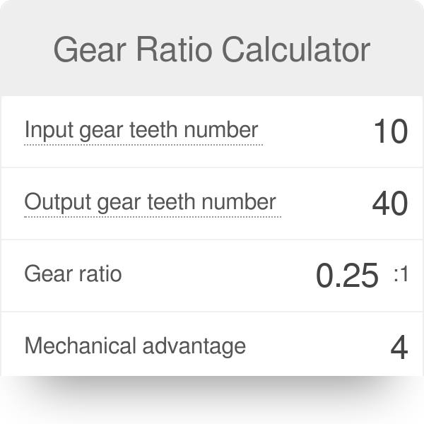
The gear ratio is the ratio of the circumference of the input gear to the circumference of the output gear in a gear train. The gear ratio helps us determine the number of teeth each gear needs to produce a desired output speed/angular velocity, or torque (see torque calculator).

We calculate the gear ratio between two gears by dividing the circumference of the input gear by the circumference of the output gear. We can determine the circumference of a specific gear in the same way we calculate the circumference of a circle. In equation form, it looks like this:

Similarly, we can calculate the gear ratio by considering the number of teeth on the input and output gears. Doing so is similar to considering the circumferences of the gears. We can express the gear"s circumference by multiplying the sum of a tooth"s thickness and the spacing between teeth by the number of teeth the gear has:

But, since the thickness and spacing of the gear train"s teeth must be the same for the gears to engage smoothly, we can cancel out the gear thickness and teeth spacing multiplier in the above equation, leaving us with the equation below:

A decimal number – expressing the gear ratio as a decimal number gives us a quick idea about how much the input gear has to be turned for the output gear to complete one full revolution.

An ordered pair of numbers separated by a colon, such as 2:5 or 1:14. With this, we can see the fewest number of turns required for both the input and output gears to return to their original positions at the same time.

From a different perspective, if we take the reciprocal of the gear ratio in its fractional form and simplify it to a decimal number, we get the value for the mechanical advantage (or disadvantage) our gear train or gear system has.

In the process of using the pump, it is often necessary to calculate the pump flow, but many people do not know the pump flow calculation formula. We will take the submersible pump and gear pump as an example to introduce the pump flow calculation formula in detail.

102 is a unit finishing constant. Pump effective power / pump shaft power = pump efficiency (generally 50% - 90%, large pump is higher) The energy obtained by the pump per unit weight of liquid is called the lift. The lift of the pump, including the suction stroke, is approximately the difference between the pump outlet and the inlet pressure. The lift is indicated by H and the unit is meters (m).

The efficiency of the pump refers to the ratio of the effective power of the pump to the shaft power. The power of the η=Pe/P pump usually refers to the input power, that is, the power that the prime mover transmits to the pump shaft, so it is also called the shaft power, which is denoted by P. The effective power is the product of the pump head and mass flow and gravity acceleration.

Submersible pump flow calculation formula: 60HZ flow × 0.83 = 50HZ flow 60HZ lift × 0.69 = 50HZ lift 60HZ power ÷ 1.728 = 50HZ motor power motor output power = Q (flow) × H (head) / 367.2 / efficiency × 1.15 motor output power = shaft power × 1.15 pump efficiency = Q × H × 0.00272 / motor power Q represents flow; H represents the head; 0.83 / 0.69 / 1.728 / 367.2 / 1.15 / 0.00272 are all coefficients.

The gear oil pump flow calculation formula is: Z——number of teeth; n——number of revolutions, revolutions/minutes; ηv——volume efficiency, for general gear oil pumps, the value can be taken as 0.70~0.90; q——the volume of the pit between the two teeth, cubic meters.

When it comes to pumping terminology, one crucial term to know is GPM — a measurement that will help you determine if you’re choosing the right pump. So what is GPM, and how do you calculate it?

GPM stands for gallons per minute and is a measurement of how many gallons a pump can move per minute. It is also referred to as flow rate. GPM is variable based on another measurement known as the Head, which refers to the height the water must reach to get pumped through the system. It is also referred to as flow rate. GPM is variable based on another measurement known as the Head, which refers to the height the water must reach to get pumped through the system.

Pumps are typically measured by their GPM at a certain Head measurement. For example, a pump specification may read 150 GPM at 50 Feet of Head, which means the pump will work at 150 gallons per minute when pumping water at a height of 50 feet.

GPM identifies the unique capabilities of a pump so you can select the right one for your specific needs. If you need a pump for a larger public area such as a golf course, marina or lake, you will need a pump with a much higher GPM than one used for your home’s well. Plus, choosing the correct pump is essential for reducing your costs and increasing your pump’s lifespan.

At GeoForm International, we are a leading manufacturer of high-quality submersible pumps, dredges, digester packages and aerators, all of which are made in the U.S. With our pump expertise, we know just how essential GPM is in the pumping and dredging industry from how much equipment costs to how long jobs will take.

When two (or more) pumps are arranged in serial their resulting pump performance curve is obtained by adding theirheads at the same flow rate as indicated in the figure below.

Centrifugal pumps in series are used to overcome larger system head loss than one pump can handle alone. for two identical pumps in series the head will be twice the head of a single pump at the same flow rate - as indicated with point 2.

With a constant flowrate the combined head moves from 1 to 2 - BUTin practice the combined head and flow rate moves along the system curve to point 3. point 3 is where the system operates with both pumps running

When two or more pumps are arranged in parallel their resulting performance curve is obtained by adding the pumps flow rates at the same head as indicated in the figure below.

Centrifugal pumps in parallel are used to overcome larger volume flows than one pump can handle alone. for two identical pumps in parallel and the head kept constant - the flow rate doubles compared to a single pump as indicated with point 2

Note! In practice the combined head and volume flow moves along the system curve as indicated from 1 to 3. point 3 is where the system operates with both pumps running

In practice, if one of the pumps in parallel or series stops, the operation point moves along the system resistance curve from point 3 to point 1 - the head and flow rate are decreased.

Pump curves are calculated based on water which has an SG of 1. If a fluid has a higher specific gravity than water, then the head will show the same, but the pressure will increase since Pressure is a function relative to fluid calculated by multiplying Head x Specific Gravity.

The presence of solids will also effect the absorbed power. Wastewater which contains sewage is typically assumed to have an SG of 1 due to the large ratio of water to solids. However slurries or sludges can have a density 2 or 3 times higher, affecting the motor power accordingly.

The pressure supplied by a pump for each application is fluid dependent and relative to fluid density thus pressure will change according to the fluid’s specific gravity

Density and pressure directly affect the power absorbed by the motor during operation. The amount of power absorbed by a motor during operation is multiplied by the SG to calculate the power absorbed.

Care must be taken where a pump curve shows a high NPSH is required. A fluid with a low specific gravity, must be checked against the NPSH required carefully.

Cavitation can occur if the inlet pressure is below that required by the pump, which can arise when the SG of the fluid is not accounted for correctly, when determining the NPSH available.

Positive Displacement Pump CurveA PD Pump curve will not be affected in the same way as a centrifugal pump curve by the specific gravity of a fluid, as flow rate will remain constant. However, the absorbed power will increase, with the pressure produced remaining fluid dependent.

Researchers have shown that mud pulse telemetry technologies have gained exploration and drilling application advantages by providing cost-effective real-time data transmission in closed-loop drilling operations. Given the inherited mud pulse operation difficulties, there have been numerous communication channel efforts to improve data rate speed and transmission distance in LWD operations. As discussed in “MPT systems signal impairments”, mud pulse signal pulse transmissions are subjected to mud pump noise signals, signal attenuation and dispersion, downhole random (electrical) noises, signal echoes and reflections, drillstring rock formation and gas effects, that demand complex surface signal detection and extraction processes. A number of enhanced signal processing techniques and methods to signal coding and decoding, data compression, noise cancellation and channel equalization have led to improved MPT performance in tests and field applications. This section discusses signal-processing techniques to minimize or eliminate signal impairments on mud pulse telemetry system.

At early stages of mud pulse telemetry applications, matched filter demonstrated the ability to detect mud pulse signals in the presence of simulated or real noise. Matched filter method eliminated the mud noise effects by calculating the self-correlation coefficients of received signal mixed with noise (Marsh et al. 1988). Sharp cutoff low-pass filter was proposed to remove mud pump high frequencies and improve surface signal detection. However, matched filter method was appropriate only for limited single frequency signal modulated by frequency-shift keying (FSK) with low transmission efficiency and could not work for frequency band signals modulated by phase shift keying (PSK) (Shen et al. 2013a).

In processing noise-contaminated mud pulse signals, longer vanishing moments are used, but takes longer time for wavelet transform. The main wavelet transform method challenges include effective selection of wavelet base, scale parameters and vanishing moment; the key determinants of signal correlation coefficients used to evaluate similarities between original and processed signals. Chen et al. (2010) researched on wavelet transform and de-noising technique to obtain mud pulse signals waveform shaping and signal extraction based on the pulse-code information processing to restore pulse signal and improve SNR. Simulated discrete wavelet transform showed effective de-noise technique, downhole signal was recovered and decoded with low error rate. Namuq et al. (2013) studied mud pulse signal detection and characterization technique of non-stationary continuous pressure pulses generated by the mud siren based on the continuous Morlet wavelet transformation. In this method, generated non-stationary sinusoidal pressure pulses with varying amplitudes and frequencies used ASK and FSK modulation schemes. Simulated wavelet technique showed appropriate results for dynamic signal characteristics analysis.

As discussed in “MPT mud pump noises”, the often overlap of the mud pulses frequency spectra with the mud pump noise frequency components adds complexity to mud pulse signal detection and extraction. Real-time monitoring requirement and the non-stationary frequency characteristics made the utilization of traditional noise filtering techniques very difficult (Brandon et al. 1999). The MPT operations practical problem contains spurious frequency peaks or outliers that the standard filter design cannot effectively eliminate without the possibility of destroying some data. Therefore, to separate noise components from signal components, new filtering algorithms are compulsory.

Early development Brandon et al. (1999) proposed adaptive compensation method that use non-linear digital gain and signal averaging in the reference channel to eliminate the noise components in the primary channel. In this method, synthesized mud pulse signal and mud pump noise were generated and tested to examine the real-time digital adaptive compensation applicability. However, the method was not successfully applied due to complex noise signals where the power and the phases of the pump noises are not the same.

Jianhui et al. (2007) researched the use of two-step filtering algorithms to eliminate mud pulse signal direct current (DC) noise components and attenuate the high frequency noises. In the study, the low-pass finite impulse response (FIR) filter design was used as the DC estimator to get a zero mean signal from the received pressure waveforms while the band-pass filter was used to eliminate out-of-band mud pump frequency components. This method used center-of-gravity technique to obtain mud pulse positions of downhole signal modulated by pulse positioning modulation (PPM) scheme. Later Zhao et al. (2009) used the average filtering algorithm to decay DC noise components and a windowed limited impulse response (FIR) algorithm deployed to filter high frequency noise. Yuan and Gong (2011) studied the use of directional difference filter and band-pass filter methods to remove noise on the continuous mud pulse differential binary phase shift keying (DBPSK) modulated downhole signal. In this technique, the directional difference filter was used to eliminate mud pump and reflection noise signals in time domain while band-pass filter isolated out-of-band noise frequencies in frequency domain.

Other researchers implemented adaptive FIR digital filter using least mean square (LMS) evaluation criterion to realize the filter performances to eliminate random noise frequencies and reconstruct mud pulse signals. This technique was adopted to reduce mud pump noise and improve surface received telemetry signal detection and reliability. However, the quality of reconstructed signal depends on the signal distortion factor, which relates to the filter step-size factor. Reasonably, chosen filter step-size factor reduces the signal distortion quality. Li and Reckmann (2009) research used the reference signal fundamental frequencies and simulated mud pump harmonic frequencies passed through the LMS filter design to adaptively track pump noises. This method reduced the pump noise signals by subtracting the pump noise approximation from the received telemetry signal. Shen et al. (2013a) studied the impacts of filter step-size on signal-to-noise ratio (SNR) distortions. The study used the LMS control algorithm to adjust the adaptive filter weight coefficients on mud pulse signal modulated by differential phase shift keying (DPSK). In this technique, the same filter step-size factor numerical calculations showed that the distortion factor of reconstructed mud pressure QPSK signal is smaller than that of the mud pressure DPSK signal.

Study on electromagnetic LWD receiver’s ability to extract weak signals from large amounts of well site noise using the adaptive LMS iterative algorithm was done by (Liu 2016). Though the method is complex and not straightforward to implement, successive LMS adaptive iterations produced the LMS filter output that converges to an acceptable harmonic pump noise approximation. Researchers’ experimental and simulated results show that the modified LMS algorithm has faster convergence speed, smaller steady state and lower excess mean square error. Studies have shown that adaptive FIR LMS noise cancellation algorithm is a feasible effective technique to recover useful surface-decoded signal with reasonable information quantity and low error rate.

Different techniques which utilize two pressure sensors have been proposed to reduce or eliminate mud pump noises and recover downhole telemetry signals. During mud pressure signal generation, activated pulsar provides an uplink signal at the downhole location and the at least two sensor measurements are used to estimate the mud channel transfer function (Reckmann 2008). The telemetry signal and the first signal (pressure signal or flow rate signal) are used to activate the pulsar and provide an uplink signal at the downhole location; second signal received at the surface detectors is processed to estimate the telemetry signal; a third signal responsive to the uplink signal at a location near the downhole location is measured (Brackel 2016; Brooks 2015; Reckmann 2008, 2014). The filtering process uses the time delay between first and third signals to estimate the two signal cross-correlation (Reckmann 2014). In this method, the derived filter estimates the transfer function of the communication channel between the pressure sensor locations proximate to the mud pump noise source signals. The digital pump stroke is used to generate pump noise signal source at a sampling rate that is less than the selected receiver signal (Brackel 2016). This technique is complex as it is difficult to estimate accurately the phase difference required to give quantifiable time delay between the pump sensor and pressure sensor signals.

As mud pulse frequencies coincide with pump noise frequency in the MPT 1–20 Hz frequency operations, applications of narrow-band filter cannot effectively eliminate pump noises. Shao et al. (2017) proposed continuous mud pulse signal extraction method using dual sensor differential signal algorithm; the signal was modulated by the binary frequency-shift keying (BFSK). Based on opposite propagation direction between the downhole mud pulses and pump noises, analysis of signal convolution and Fourier transform theory signal processing methods can cancel pump noise signals using Eqs. 3 and 4. The extracted mud pulse telemetry signal in frequency domain is given by Eqs. 3 and 4 and its inverse Fourier transformation by Eq. 4. The method is feasible to solve the problem of signal extraction from pump noise,

These researches provide a novel mud pulse signal detection and extraction techniques submerged into mud pump noise, attenuation, reflections, and other noise signals as it moves through the drilling mud.

We applied a mud pulse signal to transmit the downhole measured parameters in a Logging While Drilling (LWD) system. The high-data-rate mud pulse signal was almost completely overwhelmed by noise and difficult to be identified because of the narrow pulse width, impacts of the pump noise, and the reflected wave. The wavelet transform’s multiresolution is suitable for signal denoising. In this paper, during the denoising process of the wavelet transform, we used a series of evaluation parameters to select the optimal parameter combination for denoising a mud pulse signal. We verified the feasibility of the wavelet transform denoising algorithm by analysing and processing an operational high-data-rate mud pulse signal. The decoding algorithm was available by applying self-correlation and bit synchronization. The application results through a field application showed that the processing algorithm was suitable for the high-data-rate mud pulse signal’s process.

In Measurement While Drilling/Logging While Drilling systems (MWD/LWD), mud pulse telemetry, which generally transmitted the downhole measured signal by controlling the needle’s movement to instantly block mud flow inside the drill collar [1], remains the most widely used and reliable method for transmitting data from downhole sensors to the surface [2].

Reducing the pulse width [4] can effectively increase transmitting rates; however, the mud channel (the pipe bore filled with flowing drilling mud) causes the transmitted signal to be attenuated and further distorted [5], possibly causing the signal to be overcome by noise. Figure 1 shows the original signal waveform of 0.8 s pulse width and 0.3 s pulse width.

The principal noise source which is present is due to the pressure fluctuations caused by the process of pumping the mud. The pump pressure fluctuations can be as small as a few psi with adjusted dampers and can range up to hundreds of psi (500–600) with incorrect dampers.

Mud motor is usually used for steering operations. These noises caused by the motor’s drilling can range from a few psi to hundreds of psi and will tend to occupy the frequency band below the expected mud pump noise. However, the motor “noise” will tend to be more random than pump noise.

The signal collected in practical engineering applications such as the mud pulse signal often contains a large number of nonlinear and nonstationary components, such as trend term and mutation. These nonstationary components often reflect the important characteristic of signals.

The main function of this signal detection part is to ensure that the data transmission reliably reduces the noise components of the received signal, improves the signal-to-noise ratio (SNR) before the signal is synchronously decoded, and reduces the bit error rate (BER). Synchronous decoding locates the starting position of the synchronization to identify each frame data and the transmission parameters first, then decodes the information data according to miller’s bit synchronization and decoding algorithm and outputs the 0/1 sequence data of measurement parameters last.

Because of its low efficiency, the maximum transmit rate is about 3.14 bps, which cannot meet the demand of 5 bps in a 0.2 s pulse width. Therefore, we need a new coding algorithm for high-data-rate mud telemetry.

However, during the denoising process, lower decomposition levels led to the inefficient removal of noise interference, whereas higher decomposition levels led to the filtering out of the signal as noise, so it is essential to choose an optimal decomposition level in the denoising of high-data-rate mud pulse signal.2.2.2. Selection of Threshold Function

During the denoising process of the mud pulse signal, is the original signal and is the denoised signal. We determined the optimal wavelet basis by comparing the degree of correlation coefficient between the original signal and the denoised signal under different wavelet basis.

The significance of this formula lies in fully revealing the deviation between the two vectors. The greater the calculated ρ, the better the reconfiguration effect.3.1.3. Selecting the Appropriate Wavelet Basis by SNR

Noise also resulted from the influence of various electric motors and magnetic fields in the drilling field. The composition of the mud pulse signal was complex, and we could not determine whether the pulse was valid; therefore, it was essential to remove the baseline drift before the decoding process [22]. In this paper, we applied the wavelet analysis algorithm to remove the baseline drift of the original mud pulse signal [23].

During the simulation process, only the superimposition of pump noise is considered. The test signal can almost represent the real mud pulse signal without considering the baseline drift. Parameters for generating test signals are shown below:(1)Simulated signal: the 3 bps mud pulse signal generated by the mud pulse system in laboratory environment(2)Noise: the pump noise was sampled from an actual drilling field(3)Sample rate: 2 kHz

Test signal’s characteristics in the time domain and frequency domain. (a) Simulated signal, (b) pump noise, (c) test signal, (d) spectral characteristics of test signal, and (e) spectral characteristics of simulated signal.

According to these analyses, the wavelet transform’s parameters used for high-data-rate mud pulse signal’s denoising were decomposed at level 5 and basis db8.

Based on abovementioned conclusions, a section of the original mud pulse signal with 0.3 s pulse width (3.3 bps) in Ying-X well of XX oil field in China National Petroleum Corporation (CNPC) is shown in Figure 9. The pulse signal energy was reduced, which was almost completely obscured by noise because of the narrow pulse width, the influence of pump noise, and the reflected wave.

Based on equation (10), the calculated SNR of denoised signal is 116.2661 dB. The test results showed that the mud pulse signal processing algorithm based on wavelet transform had good adaptability, achieving 0.3 s pulse width of the original signal’s denoising.

Based on the above signal processing algorithm, since 2016, the high-data-rate mud pulse system has been carried out more than 8 field tests at different conditions in Changqing Oilfield and Qinghai Oilfield of CNPC. Table 3 shows the preset parameters’ value (in HEX). As shown in Figure 13 the signal processing system filtered out the noise, and on its left part, the decoded data are the same as the preset value.

In this paper, aiming at the process of high-data-rate mud pulse signal to acquire the transmitted downhole information, we proposed a signal processing algorithm including detecting part and decoding part.

In detecting part, based on the advantages of multiresolution characteristics of wavelet transform in signal analysis, we proposed a wavelet transform algorithm for denoising high-data-rate mud pulse signals. By comparing the correlation coefficient and reconstruction factor of the signal before and after denoising, we determined an optimal parameter combination for the denoising processing of a high-data-rate mud pulse signal and demonstrated the feasibility of the algorithm shown using actual data processing.

In the pullback operation of horizontal directional drilling pipeline crossing, the existing calculation and prediction models of pullback force are relatively simple. Each pullback force maze greatly simplifies the wellbore trajectory and fails to make a detailed analysis of the pipeline stress and external resistance when the pipeline is pulled back in each characteristic trajectory area. The factors considered are relatively simple. Therefore, it is necessary to improve the calculation method of pullback force. This paper aims to establish an improved model, enhancing the earth pressure calculation method of unloading arch and winch calculation method, and carries out an example calculation of the improved formula. Therefore, it is necessary to study the pullback process of horizontal directional drilling pipeline. Firstly, this paper analyzes the calculation method of pullback force in horizontal directional drilling; studies the calculation formula and principle of common pullback force through examples; obtains the advantages, disadvantages, and applicable scope of different formulas; and improves the calculation model of pullback force and step resistance. The numerical simulation of the step crossing process is carried out, and the variation law of local stress and strain of the pipeline and relevant conclusions are obtained. The results show that the estimates of the winch calculation method are close to the actual pullback load of the project. The earth pressure calculation method of the unloading arch and the winch calculation method are improved, and a more stable and reliable calculation formula is obtained, which provides more valuable calculation data for the actual project. In the process of pullback, the pipeline will encounter step resistance after passing through the soft and hard staggered stratum, which will suddenly increase the increment of pipeline pullback force and lead to engineering accidents. If the pullback load suddenly increases and then decreases, it may encounter similar pipeline collision accidents. At the same time, emergency measures can be taken to prevent the crossing accident and ensure the safe pullback of the pipeline.

With the continuous development of the social economy, people’s awareness of civilization and environmental protection is becoming stronger and stronger, and the requirements for a living environment are also higher [1]. In order to reduce the environmental protection problems caused by excavation when laying underground pipelines, new technology is urgently needed to meet the needs of people. Horizontal directional drilling (HDD) is to drill a pilot hole of a calibre size according to the horizontal directional drilling rig’s design line and crossing curve. Then, the drill bit is changed to a larger reamer to perform more than one pullback reaming process. When the hole diameter meets the design requirements, the full-length pipeline is finally towed back and laid. Furthermore, most of the long-distance crossing projects adopt the dual-drilling rig docking method for pilot hole construction [2–4]. As a new construction technology, HDD technology includes high construction precision, fast speed, and negligible environmental impact. Therefore, HDD technology has gradually received more and more attention [5]. HDD technology is a large-scale project combining multiple technologies, equipment, and disciplines. All aspects of the construction are linked together, and problems in one of the links will increase the cost of the project or affect the progress of the whole project [6]. HDD technology was first used in oil drilling and gradually combined with infrastructure construction and water well industry. Nowadays, it is widely used in the construction of oil and gas, municipal pipelines, etc. [7]. At present, HDD technology is also commonly used in ground source heat pump and gas layer drilling, and the application effect is good [8]. Compared with other nonexcavation pipeline technologies, HDD technology has more advantages, such as low construction cost, high efficiency, and minor surface disturbance. As a result, it has received more and more attention and has achieved better social and economic benefits [9]. As a branch of trenchless construction technology, horizontal directional drilling crossing technology has not been used in pipeline construction for a long time, but with the unremitting efforts of the majority of scientific researchers and engineers, it has made great progress since it was introduced into China in the 1970s. The construction of ground obstacles such as buildings is being widely used, and remarkable achievements have been made. Because of the outstanding advantages and mature technology of horizontal directional drilling, its application scope is expanding. Nowadays, it is used not only in the field of non-open-ended pipeline laying, but also in the fields of geology, metallurgy, petroleum, etc., and it is used in special underground space occasions like exploration and resource development of two underground sites. At present, the research on horizontal directional drilling technology has reached a certain extent. It can not only develop small- and medium-sized drilling machines produced abroad, but also expand the application field of this technology. Now, directional drilling technology not only has been applied to the laying of pipelines under complex conditions, but also can be applied to exploration and information collection in underground dangerous areas, such as laying military optical cables crossing busy roads or rivers, and automatic collection of soil data in the tunnel area after underground nuclear test. The research of horizontal directional drilling involves the research of various fields, including the research of pipeline back drag force calculation and the research of pipeline step crossing and the local stress deformation of the pipeline during the process of back drag.

Nowadays, China is in a rapid development stage, and there are more and more large-scale infrastructure projects, which will significantly promote the wide application of HDD technology. Simultaneously, the development of orientation, machinery, and computer technology also provides theoretical support for the application of HDD [10, 11]. In 2010, Chehab and Moore also put forward the mathematical method for calculating the pullback force. They considered the winch effect and the development of the pipeline. Many domestic scholars have also studied the calculation method of pullback force. For example, Hu Shilei put forward a new calculation model of separation in 2012. He not only considered the pipe bending, but also split the bending, considered the situation of pipes under different bending types and strengths, and gave calculation formulas, respectively. Through example verification, the value of pullback force calculated by the new method is more accurate [12]. At present, there is a lack of basic research on the design value of horizontal directional drilling hole/pipe diameter ratio at home and abroad for a long time, and engineering practice depends on some empirical data with a large value range for a long time. Some studies have proposed the calculation method of the bending strength of the curve section, and it is considered that the reasonable limit bending strength of the hole body can be determined only by analyzing and comparing four aspects of the limit bending strength, namely, the limit bending strength of the hole body through which the bottom hole dynamic drilling tool passes smoothly, the limit bending strength of the hole body for safe operation of the drill string, the limit bending strength of the hole body for safe operation of the pipeline, and the limit bending strength of the hole body with the lowest deviation cost per degree [13]. The pipe diameter ratio is the ratio of the diameter of the guide hole to the diameter of the pullback pipe. According to the proposed pullback load prediction method, some scholars analyzed the influence of pipe diameter ratio on the pullback load. When the value is less than 1.5, the change of pipe diameter ratio has a great impact on the pullback load, and when the value is greater than 1.7, the change of pipe diameter ratio has little impact on the calculation results of pullback load [5]. It can be seen that the pipe diameter ratio has an important influence on the pullback load. Therefore, this study analyzes the calculation method of the pullback force of horizontal directional drilling, aiming to improve the calculation models of the backdrop force and the resistance of the step crossing via a case study. To facilitate full understanding of the HDD mechanism, numerical simulation of the step hole crossing is performed. Our research helps to ensure that the directional crossing process can adjust the construction process in time according to the actual situation of the site construction, avoid crossing accidents, and effectively reduce the construction cost and risk.

In (1), is the pulling force of the drilling rig with the unit of N; is the length of the pipeline with the unit of m; ρm is the mud density with the unit of kg/m3; is the friction factor, being between 0.2 and 0.5; is the acceleration of gravity with the unit of m/s2; is the outer diameter of the pipeline with the unit of m; is the thick wall of the pipeline with the unit of m; and is the viscosity coefficient, being between 0.01 and 0.05. Note that 1.2 ∼ 2.5 times of the calculation result of the formula is the final calculation result of the drilling rig. Nonetheless, (1) is an idealized model without full consideration of all influential factors.

The 2nd method is to obtain the unloading arch’s earth pressure, which mainly analyzes the influence of the unloading arch above the pipeline on the pipeline’s total pullback load, without considering the mud buoyancy inside the borehole. This calculation is given in the following equation:

In (2), is the maximum drag force with the unit of kN; is the earth pressure per unit length with the unit of kN; is the earth pressure factor, taking 0.3; is the gravity per unit pipe with the unit of kN/m; is the friction factor between the pipe and the borehole, being between 0.1 and 0.35; is the total length of the pipe with the unit of m; is the gravity acceleration with the unit of m/s2; and is the viscosity coefficient [0.01–0.05]. Considering the drilling quality factors, the geotechnical thickness h (unit: m) and the vertical earth pressure (unit: kN/m) of the pipe top are shown as follows:

In (3) and (4), is the borehole size with the unit of m; is the borehole mass coefficient, being between 20 and 35; is the rock and soil internal friction angle: ; is the rock and soil coefficient, being 0.3; is the rock and soil bulk density with the unit of kN/m3; is the outer pipe diameter with the unit of m; and is the top rock and soil height with the unit of m. Safe pullback during construction usually means to reduce the friction force between the pipe and the hole wall and to keep the size ratio of the borehole and the pipe between 1.2 and 1.6, so the lateral earth pressure (unit: kN/m) is calculated during the pulling back process, as follows:

The 3rd method is to obtain the net buoyancy, which considers the influence of gravity and mud buoyancy on the pipeline, as shown in the following equation:

In (11), is the pipe wrap angle and is the friction factor between mud and pipe. Considering the resistance caused by the mud during the pipeline backhauling, the backhauling head is regarded as the base point, and the following equation can be derived from (10) and (11).

In (12), , . , , , and , respectively, represent the pullback forces when the pipeline is pulled back to the entry point A, the end bending point B, the end bending point C, and the exit point D; P represents the mud pressure with the unit of kN/m3; represents the movement resistance: , with the unit of kN; , , , and , respectively, represent the additional length of the pipeline, the horizontal pullback length from A to B, the length from B to C in the middle horizontal section, and the horizontal pullback length from C to D, with the unit of all these lengths being m; and represent friction factors of the ground section (0.2–0.3) and the hole (0.15–0.25); H1 and H2, respectively, represent the maximum buried depths of the ground end and the excavation end; and and , respectively, represent the entry angle and exit angle.

The calculation example of pullback force conducts the case study. First, the engineering parameters are determined according to the actual situation of the project. According to ASTM regulations (0.12–0.2) and the existing construction properties, the friction coefficient between the ground and the pipeline is set to be 0.15, the mud viscosity resistance is 0.25, and the friction coefficient in the borehole is 0.25 [15]. This study mainly analyzes three engineering cases: AA, BB, and CC, respectively. Due to the limited space in this paper, only the calculation process of AA is introduced in detail. AA is refined oil pipeline project, as shown in Figure 1.

In directional drilling engineering, drilling cuttings are flushed away by mud, improving the stability of hole wall [16]. Therefore, the method that considers the effect of mud on the buoyancy is supposed to be more suitable for the pullback force calculation. Therefore, (2) about the method of unloading arch earth pressure is improved as follows:

On the other hand, as shown previously, the calculation based on winch effect consideration gives best estimate of the force (see Table 1). Nevertheless, it can be seen from (12) that the winch calculation method is unreasonable both in the equation and the actual working condition. In fact, it can be seen from the calculation results and the actual engineering that the influence of the mud flow resistance on the back drag force of the pipeline is very small, so the calculation of this force has little practical significance. In the estimation stage of the pullback force, its size can be ignored completely, which has little influence on the calculation results. In addition, the earth pressure on the top of the pipe is also considered in the formula, but this method is too rough and far from the actual working condition. The calculation method of earth pressure above the pipe top in the earth pressure calculation method of unloading arch introduced above is relatively mature in the theory of soil mechanics. So, this method can be applied in the winch calculation to calculate the earth pressure above the pipe top. According to the unloading arch earth pressure method,

At present, China is in the climax of the development of horizontal directional crossing technology. In many cases, the calculation of pipeline pullback force depends on the empirical value, which is greatly affected by human subjective factors, and the theoretical level is far from meeting the needs of practical engineering. Therefore, it is particularly important to analyze the characteristics of pipeline in the process of crossing, especially the study of pullback load. The back drag load is affected by many factors. At present, the research at home and abroad mainly focuses on the geological conditions, trajectory curvature, mud properties, pipeline materials, and ratio of pipe diameter to hole diameter (hole/pipe ratio) but little on special construction conditions. In order to further improve the pipeline crossing theory, based on the case study of stepped hole crossing project, this section analyzes the influence of step set parameters on pipeline pullback force and pipeline mechanical properties.

In (22), D and d are the inner and outer diameters of the pipeline with the unit of m; ρ1 and ρ2 are the density of the pipeline and mud with the unit of kg/m3; and is the acceleration of gravity, i.e.,  = 9.8 m/s2. If the pipeline always keeps balance when crossing the steps, the stress of the pipeline is shown in Figure 2.

The rotation of the pipeline during back-pulling is not considered. A symmetrical model is built to reduce the computational expense, and a symmetrical constraint is imposed on the symmetrical plane to avoid rigid body displacement. The model is composed of a pipeline and geotechnical (with a step) model. When the step height is determined, the higher the contact point between the pipe and the step, the greater the step resistance. When the step height and the contact point height are constant, the step resistance decreases with the increase of step curvature. The above theoretical analysis results lay a theoretical foundation for the simulation results of stepped hole crossing in the later paper and are mutually verified with the simulation results in this paper. The rock length L is 20 m, the height H is 2 m, and the step height h is 0.1 m–0.4 m. The curvature radius r of step and joint is 0.75 m, the radius R is 0.65 m, and the wall thickness d and inner diameter R of the pipe are 0.02 m and 0.49 m. The pipeline material is X-65, the density in the elastic-plastic constitutive relation is 7800 kg/m3, the elastic modulus is 2.1e11 Pa, and the Poisson ratio is 0.3. The stress-strain data of pipeline in the plastic stage are shown in Table 3.

Drucker–Prager model is applied to the geotechnical plastic model, which is suitable for friction materials such as geotechnical materials [18]. The density, Young’s modulus, and Poisson’s ratio of geotechnical elastic parameters are 2700 kg/m3, 4.13e10 Pa, and 0.22 respectively; the friction angle β, strain rate K, and expansion angle f of D-P constitutive model parameters are 44°, 0.8, and 38°, respectively; and the corresponding plastic variables of yield stress in rock hardening parameters under 37.93 MPa, 38.2 MPa, and 38.4 MPa are 0, 0.005, and 0.08, respectively. The analysis step of stepped hole crossing and the contact attributes between hole wall and pipe are set as follows: analysis step (static general analysis step), contact surface (pipe indication), contact type (surface contact), tangential contact (penalty function), normal contact (linear contact), target surface (hole wall), and friction coefficient (0.2).

X. L. analyzed the calculation results and wrote the article; D. H. processed the data; Y. L. and Y. Z. provided the information of the construction site; L. J. and X. Y. offered useful suggestions for the preparation and writing of the paper.