pmp hydraulic pump free sample

Pmp hydraulic pump motors are suitable for high-pressure piping. They are easy to maintain and pressure well, and the installation of manual piston pump motors is suitable for both pressure and pumping.

The Knight PMP Plus Series is Knight"s newest line of variable speed metering pumps built on the industry"s most reliable and consistent platform. The high performance chemical metering system is designed to offer a wide array of flow rates and multi-functional controls to meet your pumping application needs. With the choice of peristaltic or electric diaphragm metering pumps, the PMP Plus offers the versatility to dispense a variety of process fluids or chemicals for food & beverage cleaning and sanitation, dairy farms, industrial process, and large laundry.

New multi-function electronics with high resolution variable speed control (manual adjustment or 4—20 mA input) to vary pump delivery volume depending on the application

PMP Plus Series offers the choice of Electric Diaphragm Pumps (2.8 gpm, 1.2 gpm, .6 gpm) [10.6 lit/min, 4.5 lit/min, 2.3 lit/min] or Peristaltic Metering Pumps (.6 gpm, .25 gpm) [2.3 lit/min, 1 lit/min]

The PMP Plus Peristaltic Metering Pump System features Knight¡¦s industry best peristaltic pump design that has become the bench mark for reliablity and quality for the chemical dispensing industry.

The Knight Peristaltic Pump (PMPP) PMP-8110BVS with external potentiometer is part ofKnight"s newest line of variable speed metering pumps built on the industry"s most reliable and consistent platform.

The EZO-PMP Pump consists of three main components: a cassette, a 12V motor and a control system. The actual peristaltic pumping is done within the cassette. The inner workings of the cassette are fragile and must be dismantled by hand. It has been designed to be easily detached from the motor and disassembled. The 12V motor and its control system are soldered together. Both components are designed to operate as one single unit. The control system has three main components: a keyed data and its power connector, a 12 – 24V power input and a Status indicator LED.

Before calibration is attempted, all the air bubbles should be removed from the tubing. This is done by running the pump while tapping the tubing. If air bubbles are not removed from the tubing, they will slowly group together into larger air bubbles. Over time this will lead to accuracy issues.

Mr. Ludwigson has 20 years of full-time engineering experience with projects in over 10 states across the country. He has a passion for designing state-of-the-art water and wastewater systems. Mark was the lead engineer for a prominent clarifier manufacturer for several years. He was also a trusted consultant for a top-ranked engineering firm in the water industry. He is now a design manager for industrial wastewater systems. He has brought success to a variety of water projects, including collection systems, distribution systems, pumping stations, and treatment facilities. Mr. Ludwigson has won awards for the best engineering magazine article and best paper with the Water Environment Federation.

Designed to help those that are preparing to take the PMP or CAPM Certification Exam, each post within this series presents a comparison of common concepts that appear on the PMP and CAPM exams.

PUMPCALC is a Centrifugal Pump Analysis program. It can be used to predict the performance of one or more centrifugal pumps, at various impeller sizes, speeds and series or parallel configurations.

The main data needed for running PUMPCALC is the pump performance data. This consists of sets of values of Flow rate (or capacity), Head and Efficiency for a particular pump, for a specific impeller size and speed. Normally, you will need to get this information from a pump catalog. The number of sets of Flow, Head and Efficiency values are limited to between 3 sets of points (minimum) and 15 sets of points (maximum). The data points taken off of a manufacturer"s pump curve must cover the entire range of flow rate permissible for the specific pump. Extrapolation can be made but may result in inaccurate results. Pump data files are saved under a name with PMP file extension, such as Compton.pmp

In addition to the three columns of data for Flow rate, Head and Efficiency you may also specify the pump impeller size, speed and the number of stages in this pump. After entering all data, choose File/Save from the menu bar and save the pump curve data in a file name of your choice. The Advanced... button above is for entering a single design point data for a pump, in order to create a typical pump curve. For example, if the desired design point is at 1000 gal/min, 2500 ft head at 80% efficiency, you may enter this data for PUMPCALC to automatically create a pump curve based on this design point, as shown in screen below.

After entering data for the design point as above, and selecting a name for the pump file, click the Create file button. PUMPCALC will automatically create a pump curve for the design point specified as indicated in the screen below. It can be seen that the pump curve data have been created around the best efficiency point (BEP) specified above.

The Interpolate.. button located on the right side of the pump curve screen is used to interpolate data from a given pump curve. Upon clicking this button the following screen is displayed:

From this screen, you may interpolate the pump curve data for different flow rates. For example, at a flowrate of 1100 gpm, the interpolated head and efficiency are 2369.26 ft and 79.27 % respectively. The brake horsepower for water is also calculated and displayed as indicated above.

There are four main features of PUMPCALC, as indicated by the four buttons arranged vertically down on the left hand side of the main screen, shown above. The button titled Single Pump is for calculating the performance of a single pump, determining its performance at different impeller diameters and speeds and generating a graphic plot of the Head versus Capacity, Efficiency versus Capacity and BHP versus Capacity curves. Also, for a given Design Point (Q-H value), it can be used to calculate the new impeller size or speed.

The third button titled Viscosity Correction is for predicting the performance of a pump when pumping viscous liquids. For high viscosity liquids, the given water performance curve is used in conjunction with the built-in Hydraulic Institute charts to estimate the viscosity corrected pump performance. The resultant performance curves may be plotted on the screen as well the printer.

The fourth button titled System Curve is for calculating the System Head curve versus the pump curve, when the pipe system characteristics are given. The point of intersection between the pipe system head curve and the pump curve can be determined using this option. For a given pipeline diameter, length and elevations, the system head curves can be generated for different liquid properties and the point of intersection of the pump curve and the pipeline system curve can be determined. Screen graphics of the combined pump performance versus the system curve are also generated.

Using Affinity Laws, the pump performance at different impeller diameters and speeds can be calculated, from the given pump curve data based on a particular impeller size and speed. Also, for a specific design point( head and capacity values), the program can predict the impeller size or pump speed required, based on the existing impeller size and speed. Clicking the Options.. button in the above screen displays the following window for specifying the required design point (Q-H values)

A family of pump Head versus Capacity curves may be generated from given pump data at various impeller sizes or pump speeds, using the Affinity Laws. The results of the above are shown in a graphic plot as follows:

Clicking the Multiple Pumps button from the main screen displays the following window for entering pump data to calculate the combined pump performance in Series or Parallel configuration.

After entering the data for pumps, clicking the OK button will display the calculated results for combined pump performance. The screen graphics of the combined pump performance will also be displayed, based on the plot option chosen from the following screen:

Clicking the Viscosity Correct button displays the following window for inputting the pump and liquid data for performing the viscosity correction, using the Hydraulics Institute chart method.

Enter the file name of the water performance curve and the file name for storing the viscosity corrected performance data. Press F3 to view a directory listing of available pump data files to choose from. Only those pump files with a PMP extension will be displayed. Change the default extension from *.PMP to *.* to view all files. The file name for the viscous curve, by default has the letters VSC added to the pump file name. For example, if the water curve is Pump1.pmp then the viscous curve will be shown as Pump1vsc.pmp

The viscous performance calculated requires the use of the Best Efficiency Point (BEP) from the water curve. This is defined as the point on the water performance curve with the maximum efficiency. The flow rate, head and efficiency at this point on the curve is used as the starting point for viscosity corrected performance calculations. The BEP values may be specified in the appropriate fields or you may have PUMPCALC calculate the BEP by interpolation. After entering all data, click on the Calculate button to start calculations. Based on the Hydraulic Institute Charts, the water performance curve will be corrected for the given liquid viscosity. The water performance curve and viscous performance curve calculated will shown side by side in spreadsheets as shown below:

It must be noted that the results displayed are for only the four sets of data(60% BEP, 80% BEP , 100% BEP and 120% BEP) for both water curves as well as the viscous curves, in accordance with the Hydraulic Institute method.

Once the viscous performance is calculated, additional points on the viscous curve can be determined by interpolation. If the water performance and the corresponding viscous performance are desired at a particular flow rate, enter this value in the Flow rate field as shown above and click the Calculate button. The performance on both curves at the specified flow rate will be calculated and displayed on the spreadsheets, in a highlighted color. Similarly, additional data points on both curves can be calculated. Remember that extrapolating beyond the limits of the performance curve, though feasible, may be inaccurate. Due to the nature of the Spline Interpolation method used, extrapolation may, in some cases yield incorrect results. However interpolation is generally quite accurate. The calculated viscous performance curve is saved in a data file as shown in screen above. This curve information may subsequently be used with Single Pump option to determine other performance characteristics using affinity laws.

Clicking the System Curve button on the main PUMPCALC screen displays the following window for inputting the pump and pipe data for calculating the System Head curve and operating point. The latter is the point of intersection between the system head curve and the combined pump performance curve. The liquid properties data input screen should also be checked to ensure that the correct liquid data (specific gravity and viscosity) is used in these calculations.

For calculating the pipe system head curves, the pipeline data (distance, elevation, diameter, wall thickness and pipe roughness) are input and stored as a data file. The liquid specific gravity and viscosity are input under the separate Liquid screen, from the pull down menu on the main PUMPCALC screen. The pump suction pressure, pipe delivery pressure, maximum allowable pipe pressure and the pressure drop formula are also input in the screen above.

Alternatively, instead of pipe data above, the system head curve may be directly input. This option allows you to enter the Flow rate versus System head data for plotting against the pump head curve. If the System Head curve data is input, PUMPCALC ignores the pipe data and uses the system head curve data, without calculating the pressure drops.

When used with the given pipeline data, in the absence of system head curve information, pipeline pressures are calculated for various flow rates to generate the System Head curve. Hydraulic calculations are performed based on the chosen pressure drop formula, such as Colebrook-White, Moody, Hazen-Williams, MIT or Miller equation for isothermal conditions of flow. The output consists of the pump operating flow rate, discharge pressure, efficiency and horsepower at the operating point. Screen graphics of the combined pump curve and system head curve are also generated as shown below:

WARNING: Although PUMPCALC provides an option of extrapolating pump curve data beyond the values input by user, this can some time result in inaccurate results. Use this option with caution!

Always try to include sufficient points (up to a maximum of 15 sets) from the manufacturer"s pump curve data covering the full range of flow rates anticipated. Do not depend on PUMPCALC to extrapolate performance data beyond the range of values input!

Please note that all pump data files should conform strictly to the specified format as explained in the user manual. Each pump data file consists of flow rate, head and efficiency values stored in a comma delimited, text file format. You may view a pump data file in a text editor, such as the Windows Notepad. However, to edit or make changes to a pump data file, use only the spreadsheet editor provided with the PUMPCALC software. Refer to the sample data file named DEMO.PMP included with PUMPCALC.

Data files are created using the built-in spreadsheet and saving the data in a text file. If you want to use a text editor, such as Windows Notepad, make sure the data format strictly conforms to the format shown in the sample pipe and pump data files. The spreadsheet approach automatically takes care of the format.

From the main screen menu bar, choose File followed by New and a blank spreadsheet opens up. This window is used to input the pump data to create a new data file.

Enter the pump information namely flow rate, head and efficiency under appropriate columns, such as 0,3185,0.01 etc. as shown in the first screen at the beginning of this document. A maximum of 15 points (rows of data) are allowed in the pump data file.

You may obtain a screen plot of the pump curve by clicking the Plot icon. If a printed graphic is also required, click on Printer output button. Make sure you save the pump curve data first, before clicking the Plot button. You may also calculate interpolated values from the pump curve by clicking the Calculate button on the right side of the pump curve spreadsheet.

For the System Curve option, you may want to create a pipe data file or a system curve data file. This is done by double-clicking on the pipe file name in the Pump Curve System Curve Analysis screen. A screen will be displayed with a spreadsheet for entering the pipe data as shown previously.

We welcome comments and suggestions from users. Please give us your thoughts on how PUMPCALC can be improved further. Our goal is to make this software the most user-friendly program available.

REICH’s axially pluggable RCT flange coupling is the answer to the question of an optimal drive solution for connecting hydraulic pumps and diesel engines. Above the operating speed critical resonances can be shifted due to the torsional stiffness of the RCT coupling and an operation of your application is possible without the occurrence of dangerous torsional vibration amplitudes.

A wide variety of gear teeth as well as SAE flywheel dimensions can be selected for the RCT and allow, for example, backlash-free clamping connection with pump shafts and uncomplicated mounting on combustion engines and hydraulic pumps. Individual special designs can be configured to suit your application on request.

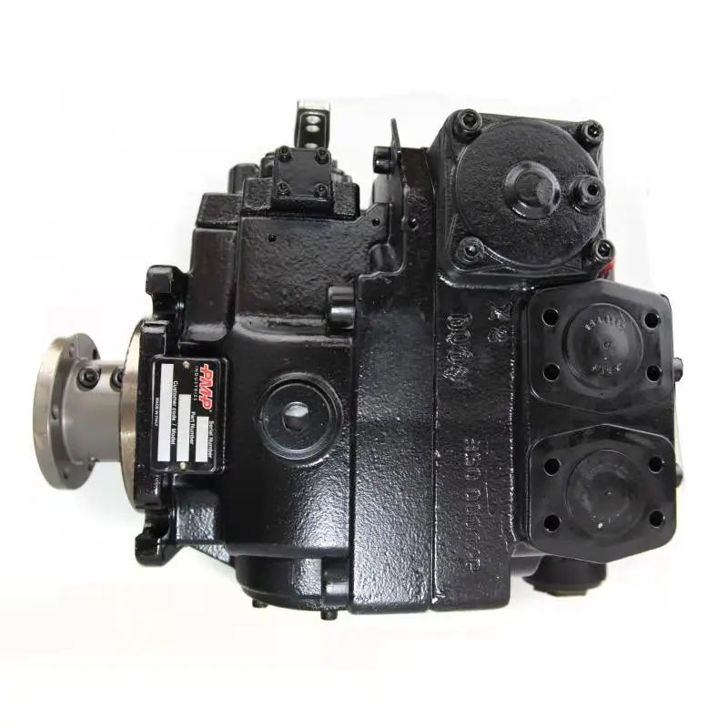
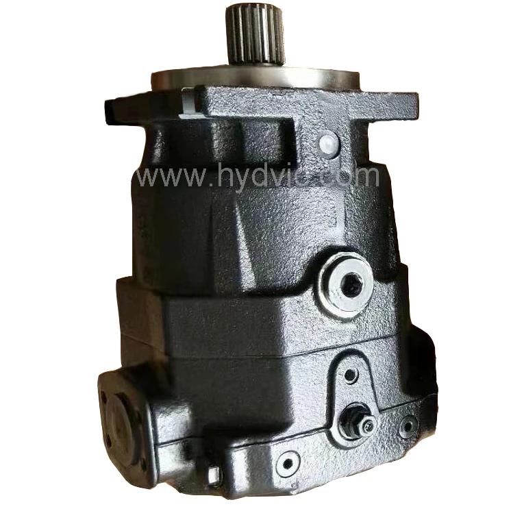
The core design concept of PMP variable displacement pump is: efficient and durable, using high-quality materials, tight tolerances and high-precision equipment manufacturing to ensure the best quality of products. The element geometry is fully optimized to reduce wear and the most efficient fluid dynamics. The overall structural design of the product also ensures that it will not deform under external pressure and load, and can maintain this efficiency even under high pressure conditions. Different sizes of PMP axial piston pumps have different control options (for example: manual, electric ratio), which can be combined with other pumps.

Construction machinery-involving road rollers, pavers, milling machines, graders, road mixers, spreaders, skid steer loaders, busy at both ends, cranes, crawler cranes, aerial work vehicles, flatbed trucks, cement mixer trucks , Concrete pump trucks, bulldozers, railway locomotives, oilfield logging / cementing / workover / sand mixing equipment, airport vehicles, port equipment, coal mining machinery, trenchless drilling rigs, rotary drilling rigs, anchoring and prospecting machinery, forklifts, Hydraulic systems such as rice harvesters and large and medium horsepower tractors.